Eggsperimenting

At a young age, I internalized the Pokémon mantra: Gotta catch ‘em all. For me, that took the form of animal rearing: mice, hermit crabs, guinea pigs, and eventually, an ever-growing flock of backyard chickens. Of all of them, chickens really stuck. In particular, they provided an ideal intersection of variety, personality, and scale, each having distinct temperaments.

College, then years of yardless housing, temporarily interrupted that period of homesteading. And now, many years later, with a modest yard of my own, I finally have the opportunity to regain that dream. But this time, with more (data) science.

Phase 0: Preparing for the Eggsperiment

At the end of January, I drove around the state of Virginia collecting eggs from three different flocks in an effort to source a diverse array of chicken stock. To incubate them, I sourced an old, but high quality Brinsea incubator back from my high school days as well as a budget, brand-new model to begin the incubation process.

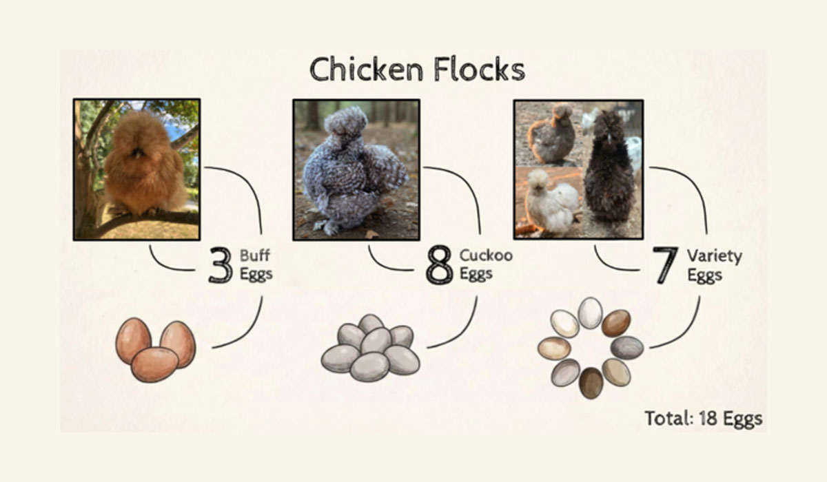
Parents from the three source flocks and the number of eggs incubated from each: 3 buff (orange), 8 cuckoo (gray and speckled), and 7 variety (a mix of spotted, chocolate, etc.). Infographic generated using Google Slides AI design tools. Chicken images are sourced from respective flocks.

Although the parent flocks had many similarities in breed and size, egg characteristics were not uniform. Attributes like egg size, shell thickness, porosity, mass, and coloring varied meaningfully from bird to bird.

These eighteen eggs were divided between two incubators: seven were placed in the Brinsea and 11 in the budget model incubator.

To make tracking each egg more intuitive (and a bit more entertaining), I named all eighteen after characters from Brandon Sanderson’s Cosmere–  a collection of interconnected book series beloved by me and set within the same universe. In an effort to manifest hens, I chose all female characters. No longer would they simply be egg_03 or egg_14, but Vin, Jasnah, Shallan, Tress, and others, adding to the weight I personally felt along each egg’s probabilistic journey. One non-Cosmere name was put in the mix at my fiancé’s request, Karlach, a subtle nod to the popular video game, Baldur’s Gate 3.

A wide sample of Cosmere novels that inspired the egg names.

This small narrative device helped me stay engaged throughout the rigorous data collection process and made understanding the viability curves and physical traits of each egg much easier to remember. With names, the eggs were no longer just abstract data points but part of a larger story.

After the preliminary steps of a daylong sojourn across Virginia, careful naming deliberation and incubator setup, incubation began.

Chicken egg incubation typically lasts 21 days culminating in a lockdown period at Day 18 where environmental changes are “locked down”– humidity is heightened and egg turning stops in preparation for the hatch. Throughout the first 18 days of incubation, a technique called candling can be applied where a candle (or light) is shown into eggs to see their internal development. This helps determine whether an egg is fertile or infertile and in some cases whether development ceases over the incubation period.

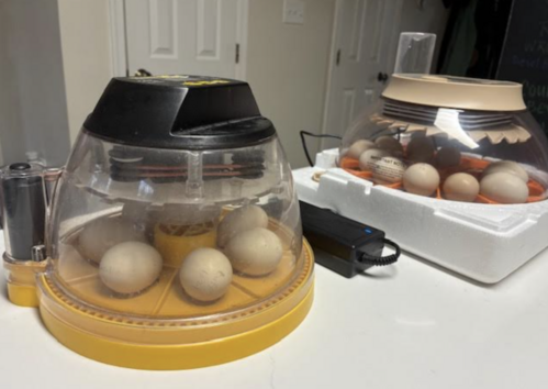
18 eggs split between old, high-quality incubator (left) and new, budget incubator (right)

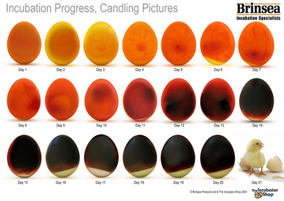
This day by day candling guide came with my Brinsea incubator and outlines the expected embryonic development progression.

In theory, egg development is quite predictable. Early on, veins begin to appear and soon those veins darken and expand. But in practice, candling is far less straightforward than an image like this may suggest. Lighting, angle, and even shell pigmentation can drastically affect interior visibility and obscure embryonic development.

This ambiguity introduces uncertainty. And that uncertainty is the main motivation for this work. If candling is inherently a subjective measure, could a more probabilistic method be introduced to improve prediction?

To answer this question, I performed the Eggsperiment. It was structured into four main phases. First, visual model training, then application of the vision model to my 18 eggs across incubation days. Third, quantitative analysis and categorization of physical attributes. And finally synthesis of results– this involves combining visual fertility signals with physical ratings, comparing them to true hatch outcomes, and evaluating predictive performance using a logistic regression model.

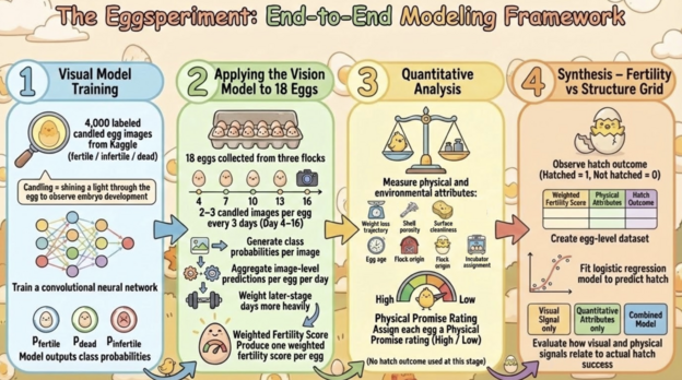
Workflow of the visual, quantitative, and post-hatch modeling process. Image generated using Google Slides AI design tools.

Phase 1: Visual Modeling

The first phase of this, visual modeling, was only possible due to a public Kaggle dataset of 4,000+ candled chicken egg images.

labeled across three classes: fertile/ infertile/ dead. This dataset provided a strong training foundation for the model that could be generalized to external data like my own eighteen eggs.

Using this dataset, I trained a convolutional neural network with a standard 80/20 train/test split. The goal of this model was not to be perfectly accurate, but rather to create probability estimates per egg per day. These probabilities would later be aggregated over time and combined with physical egg attributes to inform an overarching viability assessment prior to hatch day. After hatch outcomes were observed, these same fertility probabilities were incorporated into a logistic regression model to evaluate how well pre-hatch indicators predicted actual success.

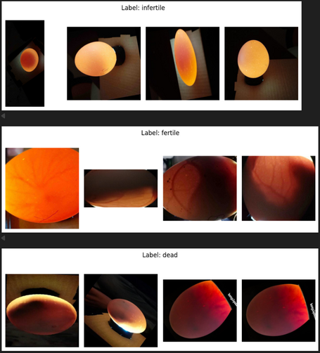
Kaggle dataset sample images in each class: infertile, fertile, and dead.

To a keen eye, many of these images can be mapped to their true labels even by a human observer. Some fertile eggs are quite obvious and the same is true for some infertile ones. But not all egg images are as straightforward. Arrested development can prove particularly challenging to identify. These eggs often share many of the signs of life of a fertile, developing egg. But slight variation in angle or lighting can make classification ambiguous. And it is in this ambiguity that this model shines, being able to capture faint signals and produce probability estimates rather than simply imposing a binary judgment.

On the test set, the model achieved an overall accuracy of 96% and an AUC of 0.91, indicating strong class separation despite variability in image type and quality across the three classes. While not perfect, the model performed strong enough to justify its use as a predictive tool.

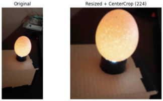
Example of standardizing training data image size through standard cropping

Before training the model, some data preprocessing was required, including image standardization. Training images had differences in size and framing. To mitigate this noise, all images were cropped and resized to a standard format. This preprocessing step is crucial in ensuring the model focuses on fertility signals rather than noise generated from image type.

After training, the network produced over 400 dimensional feature representations contributing to predictions. These are not human readable variables but instead abstract patterns discerned from pixels. Although a powerful model, these “features” are incredibly difficult to interpret, highlighting its black box nature.

Picking one of the most predictive features, Feature 343, provides some insight into what the model is picking up on.

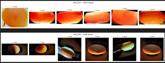
Examples of images with high and low values for Feature 343.

High values correspond primarily to fertile eggs, while low values correspond to dead eggs.

Fertile eggs have higher values for Feature 343 where dead eggs score low. A human might describe this feature as one that keys in on slight vascularity, orangish red undertones, and early embryo appearance. By contrast, those dead eggs with lower Feature 343 values often look much darker, sometimes asymmetrically, with limited embryo presence in the dark part of the egg. It is important to note that the model does not make these distinctions in the same way a human might. Instead of “seeing vascularity”, it is responding to pixel patterns that hold the meaning of “vascularity” to human observers. This example does an excellent job of showcasing the pros and cons of the model. While successfully capturing visual distinctions, reasoning can still appear subjective and difficult to define by humans.

Phase 2: Applying the Vision Model to my 18 Cosmere Eggs

To apply the model to my eggs, I took 2-3 images of each egg every 3 days under consistent lighting, beginning on day 4 and going through day 16. The trained model then assigned class probabilities to each image, as seen below.

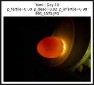
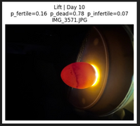
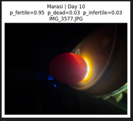
Day 10 candling images of select eggs with model-assigned class probabilities

How to read this: In this Day 10 example, Yumi was assigned a 0% probability of being fertile, 2% probability of being dead, and 98% probability of being infertile.

While images were taken in a consistent environment, minor differences in photo consistency introduced variability. If you ever try taking the same iPhone photo in the dark 54 times, you will learn that it is near impossible to eliminate variation.

In contrast to structured, quantitative data, images introduce noise. An image of an egg that looks nonviable could simply have been captured at a bad angle, with a glare, or with a blur. To mitigate these effects, I averaged the probabilities from the 2-3 images captured per day per egg, reducing the influence of photographic noise in favor of fertility signal.

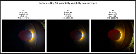
High Variation Fertility Probabilities of Karlach on Day 10

How to read this: These three Day 10 images of Karlach showcase the impact of lighting and focus. These images, taken within seconds of each other,  produce fertility estimates ranging from 2% (right) to 92% (left).

Early in incubation, fertility signals were weak, averaging close to 0% on Day 4. This reflected the low levels of vascularity and embryonic development early in incubation. At this stage, all eggs were indistinguishable from one another in terms of fertility. All were classified as Low Fertility, or what I deemed Minor Characters, aligning my labels with their Cosmere-inspired names.

By day 7, clearer patterns started to emerge and fertility was more detectable. As signs of life became more evident, the model was able to produce more differentiable probabilities. From this, I identified three key narrative groups: the Minor Characters, with consistently low fertility signals, the Cliffhangers, eggs with moderate or highly variable fertility signals, and the Protagonists, who had the strongest fertility signals.

These categorizations are a bit quirky, but help serve as common terminology throughout the Eggsperiment that translates disparate data into recognizable groups and patterns.

Over time, these groups continued to diverge, with actively developing embryos and arrested or infertile eggs moving further apart in signal strength. What began as a uniform group of low fertility eggs continued to evolve into distinct probabilistic directions and narrative arcs.

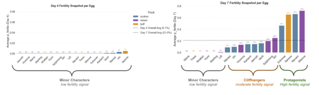
Comparison of Day 4 and Day 7 fertility probabilities averaged per egg. This illustrates the uniformity and the emergence of three narrative groups.

Phase 3: Quantitative Analysis of Physical Attributes

While the visual model is a strong start to predicting egg viability through internal development, I wanted to add a more interpretable layer grounded in measurable physical characteristics. Candling captures the egg’s internal structure, but it does not take into account external traits, like shell porosity, egg age, cleanliness or weight loss. These are meaningful attributes that can contribute to egg viability and better inform predictions.

Factors outside of visual development affect hatchability. And while visual development (detected by the vision model) is a prerequisite for viability, it is not a guarantee of hatch.

To quantify these physical factors for each egg, I collected structured data in a CSV of measurements seen below. Many of these traits were selected based on common breeder wisdom and hatch lore from online chicken forums.

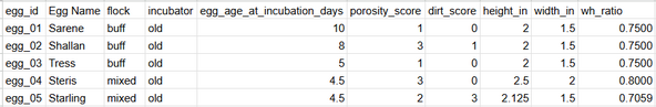
Example of static physical measurements collected for each egg.

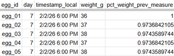
Longitudinal weight measurements of weight (typically moisture) loss over time.

Weight changes were of particular interest since a successful incubation period is characterized by controlled moisture loss, targeting 12-15% loss from starting weight. Too little moisture loss can result in a small air cell, while too much can dehydrate the embryo.

Shell porosity and shell surface cleanliness can affect egg viability. More porous eggs have greater moisture loss and dirty eggs can increase bacterial exposure and mortality risk.

Measures of flock origin and incubator assignment are recorded to account for environmental differences between eggs and habitats. Egg age is recorded as eggs past 7-10 days at the start of incubation decline in viability.

Below, I do basic exploratory data analysis to visualize distributions physical attributes across eggs, incubators, and flocks.

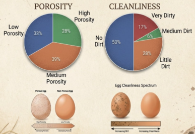
Distribution of shell porosity and surface cleanliness across the 18 eggs.

Data and pie charts by Nikki Petzer, formatting and images generated using Google Slides AI design tools.

Fourteen eggs show no to little signs of surface dirt and thirteen eggs have low to medium porosity– both boding well for hatch viability.

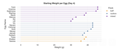
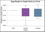
Starting Weight per Egg and Flock, Distribution of Egg Proportions by Flock

Egg sizes and shapes varied by flock with the three buff eggs having significantly smaller size than cuckoo and mixed. Buff eggs are tightly distributed in both shape and size. Eggs from the mixed flock have some of the largest eggs, but also the most variable, likely due to mixed heritage.

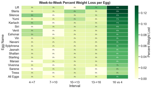
Percent weight loss by egg across incubation intervals and for full period.

How to read: Between days 4 and 7, Silence lost 6% of weight. Between days 7 and 10, Silence lost 0% of weight, and so on. From Day 4 to Day 16, Silence lost a total of 12% weight.

Unfortunately, I began weight measurements late, beginning on Day 4, and since I collected these every three days, the last collection was on Day 16, leaving the full Day 1-18 weight loss unmeasured. As a result, total moisture loss required some extrapolation.

Across the observed 12-day period (Day 4 to 16), weight loss ranged from 5% to 13%. Assuming a roughly constant rate of moisture loss, the projected total loss across the full period ranged from 7% to 18%, averaging at 12.5%, well within the target range.

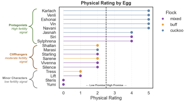
Using these quantitative measurements, I assigned a Physical Rating score to each egg, ranging from 1 to 5. A low Physical Rating reflected low viability promise and a high Physical Rating indicated high promise. Negative traits like dirtiness, high porosity, outlying weight loss (too high or too low),  egg shape, and egg at incubation all contributed to this score.

An egg like Yumi, that was given a maximum dirtiness and porosity score, outlying egg weight loss, and irregular weight loss was categorized as low promise. Conversely, an egg like Venli, with a clean shell, low porosity, average weight loss, average egg shape, and low egg age, was assigned a high promise score.

The resulting ratings are visualized in the lollipop chart below, where eggs are bifurcated into low or high promise groups. These groupings mirror the narrative groupings introduced in the visual model and will be used in combination with visual score groupings later on.

Computer Vision based Fertility Curves

How to Read Example: top left graph “Karlach’s average probability of fertility on Day 4 was 0%; on Day 7 was 20%, on Day 10 was close to 50%”… and so on

Phase 4: Image-Based Fertility meets Physical Promise

Up until now, I have examined visual development and physical qualities independent of one another. The visual model measures evolving fertility signals over time, while the quantitative analysis was an assessment of each egg’s physical qualities’ promise.

When viewed longitudinally, the fertility probabilities from the vision model form a curve. Some eggs have steadily rising signals, while others plateau early and some fluctuate. These curves illustrate the dynamicness of fertility signals.

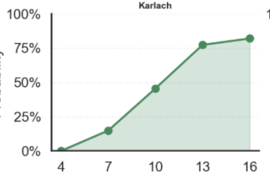
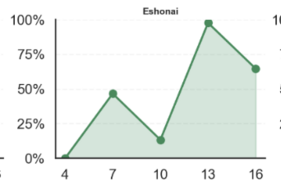
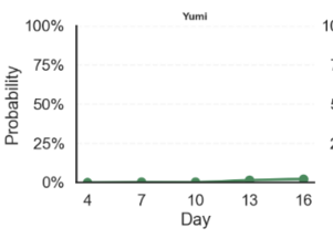
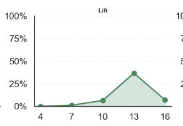
Computer Vision based Fertility Curves by Egg Across Incubation Days

How to Read Example: top left graph “Karlach’s average probability of fertility on Day 4 was 0%; on Day 7 was 20%, on Day 10 was close to 50%”… and so on

A variety of fertility scores are displayed above with Karlach illustrating a steady fertility signal increase, Eshonai showing constant fluctuation, Yumi an early plateaued egg, and Lift, a developing egg that stopped developing over time.

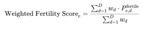
I then averaged the vision model fertility probabilities across all observation days, weighting later-stage predictions more heavily. This produced a single fertility measure per egg over the full period.

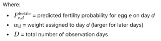
Viewed through this single snapshot lens, many of the early Minor Characters from Day 4 and Day 7 remain low in fertility signal for the full period, including Steris, Shallan, Yumi, and Tress. Other early low fertility eggs like Starling and Venli, gained a greater signal later in development, joining the Cliffhangers group. Some eggs like Karlach and Silence maintain their early strong fertility signals throughout incubation, solidifying as Protagonists.

Computer Vision based Weighted Fertility Probability per Egg (based on full period)

How to Read Example: “Sarene has a total 59% weighted fertility probability across all days, firmly placing her in the category of “Cliffhangers”, those eggs with an overall moderate fertility signal”

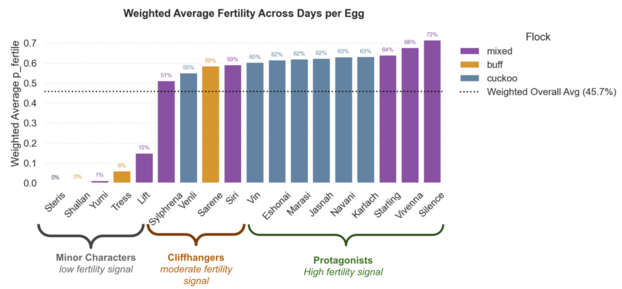
The weighted fertility score can now be evaluated alongside each egg’s Physical Rating for a fuller picture of egg viability. This cross-section reveals not only which eggs are visually developing thus far, but also whether the egg has a strong physical foundation. The grid below showcases the alignment and misalignment of these two approaches, with the x-axis measures computer vision modeling outcomes and the y-axis indicating physical rating results.

Overall Egg Viability Groups

How to Read Example: “Silence is categorized a cliffhanger. It has the highest modeled fertility signal of all eggs, but moderate to low physical rating, making its viability uncertain.”

Five eggs emerged as Minor Characters, eggs that either had no signs of fertility from Day 1, or had clear signs of arrested development later on. In these cases, both the visual and physical assessments align towards no low viability.

Seven eggs belong to the Cliffhangers category, meaning that the two methods have disagreement in viability. More commonly, an egg is assigned high fertility by the computer vision model but low promise via physical rating. In these instances, I give favor to the fertility signal. Poor physical traits like an odd shape or dirty shell do not prevent fertility or viability but are more so supplemental information. Venli and Sylphrena fall into the inverse Cliffhangers, eggs with strong physical promise but moderate or variable fertility signals. Although clearly fertile, it is difficult to tell visually whether these eggs have arrested development. These eggs are truly cliffhangers, and it feels like a toss up on whether they will hatch.

Excitingly, six eggs emerge as Protagonists, with both assessments agreeing on fertility and physical promise. Eggs like Karlach and Eshonai in particular are the strongest candidates for hatch.

In the final phase of the Eggsperiment, I will reconcile these predictions with true hatch day outcomes. By comparing these, I can assess the value of each method and build towards an explainable viability model.

Phase 5: Results Synthesis and Interpretation

Anticipation built between Day 20 and Day 21 with the first external pips (the initial crack in the shell) coming as early as the morning of Day 20. Literature suggests that the expected pip to hatch duration is typically 12 to 24 hours, with much of that time spent resting before final hatch exertion.

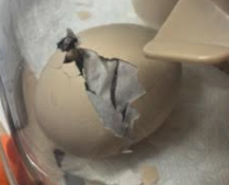
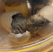
Pip to Zip to Hatch

Ten of 18 eggs ultimately hatched. Five of these 18 were confidently predicted to be non-viable due to clear infertility or arrest signals and did not hatch as predicted.

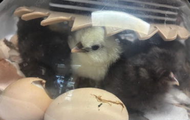
Day Old Chicks

The image below shows the time between first external pip and full hatch, with a few approximations when true times were not observed. Two extreme outliers, Starling and Sarene, left me on the edge of my seat, taking over 36 hours to hatch and one requiring minor hatch assistance. On average, pip-to-hatch time took 18 hours, but this was skewed by extreme outliers, with the median pip time being 14 hours, more in line with established expectation.

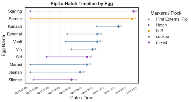
Time from First External Pip to Hatch

How to Read Example: “Starling pipped at 9:00 AM on Day 20 and fully hatched 37 hours later at 10:20 PM on Day 21.”

Mapping true hatch labels to my fertility-physical grid, it is clear that the categories were highly informative but not perfect.

Navani is the most notable exception– a strongly viable egg, both by fertility signal and physical rating, but did not hatch. To add context, when I manually inspected it on Day 16, I detected signs of late-stage arrested development that the computer vision model failed to capture. This is an interesting example of human judgment outperforming the model, showcasing potential weakness in the computer vision model.

On the flipside, all firmly classified Minor Characters did not hatch, aligning with prediction, with the exception of Sarene, a borderline Minor Character, that hatched against the odds. Among the two Cliffhanger groups, Vivenna and Sylphrena did not hatch. These two had some of the lowest scores in their respective groups. All other (higher rated) Cliffhangers hatched.

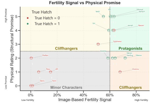
Overall Egg Viability Groups with True Hatch Outcomes

How to Read Example: “Silence was categorized a cliffhanger and did hatch. It had the highest modeled fertility signal of all eggs, but moderate to low physical rating.”

Using hatch outcome as the dependent variable (P_viable), I fit a logistic regression incorporating physical attributes and vision model fertility probabilities. Note that with a mere 18 observations and strong multicollinearity among variables, this analysis is intended as directional and narrative rather than scientifically definitive.

Images are provided below in order to interpret the logistic model. The coefficient plot gives insight into direction and general strength of effects. Eggs belonging to the cuckoo flock are by far the strongest indicator of hatch success. In contrast, lower cumulative weight loss (low weight loss for the full measured period) had the strongest negative association with hatch rate.

The second chart, odds ratios, is a human-readable version of the feature effects. Each bar shows how much more or less likely an egg was to hatch based on a feature’s presence. The exceedingly high value for cuckoo flock (>100) shows that this feature is a near hatch success guarantee. This is more likely a result of sample size than an extrapolatory truth. Similarly, other feature effects that are counterintuitive, such as dirtier and older eggs being associated with higher hatch rates, are almost certainly due to noise in this small dataset and are not generalizable.

Finally, I plotted predicted probability of viability against true outcomes. The model easily identifies successful hatches, with no false negatives. Conversely, the wider red curve suggests difficulty in distinguishing a truly non-viable egg from a viable one, producing greater false positives.

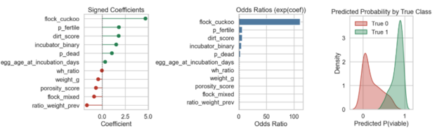
Model Diagnostic Charts

Visualizing logistic model prediction across incubation days, I plotted viability by flock and incubator. Overall, incubators performed similarly, with the hatch rate of the older Brinsea being 57% compared to 54% in the newer model. Flocks had high viability variability, with the cuckoo flock having a total 75% hatch rate compared to 43% and 33% from mixed and buff, respectively.

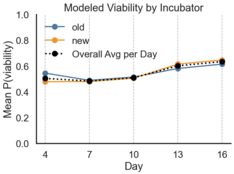
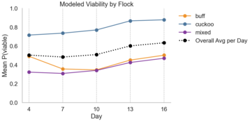
Viability Probability per Day by Incubator and Flock

How to Read Example: “On Day 4, the model predicted a 55% change of hatch for eggs in the old Brinsea incubator and 50% for eggs in the new, budget incubator.”

Overall, the Eggsperiment was a joyful intersection of two passions, data and chickens. And it was an opportunity to highlight the different approaches in which we can predict outcomes, through deep learning, quantitative analyses, and human discernment. Each approach had its own strengths and weaknesses. The vision model detected subtle pixel patterns that were not discernible to the human eye and the physical rating grounded the predictions in a more tangible and interpretable structure.

In the end, the modeled outcomes aligned closely with the true hatch outcomes. Although not perfect, predictions were strong enough to demonstrate how models can layer upon one another and complement human discernment, working to reduce uncertainty in a measurable way.