Showing posts with label ibm. Show all posts

Energizing a vacuum-tube flip-flop module from a 1948 IBM system

In 1948, IBM introduced the 604 Electronic Calculating Punch. This machine was a programmable calculator, about the size of a double refrigerator. It was not quite a computer, but was programmed by plugging wires into a plugboard. This machine read numbers from a punch card, performed up to 60 calculations on these numbers, and then recorded the results by punching holes in the card.1 It processed 100 cards per minute—over one card per second—and IBM advertised it as the equivalent of 150 engineers. The machine rented for $550 a month, making it very popular, with over 5600 units produced.2

The IBM 604 Electronic Calculating Punch. Photo from Ed Thelen's IBM 604 page.

The IBM 604 Electronic Calculating Punch. Photo from Ed Thelen's IBM 604 page.

The IBM 604 came out just after the transistor was invented, too early to use transistors. At the time, calculators and computers were moving from slow electromechanical components to fast vacuum tubes. One of the innovations of the 604 was to combine a vacuum tube and its associated circuitry into a pluggable module. Along the left side of the photo above, you can see rows of these modules with the handles sticking out, making it easy to replace a faulty module. More modules are behind the silver metal covers. In total, the IBM 604 used about 1300 vacuum tubes.

The photo below shows a pluggable tube module, with a vacuum tube underneath the insulated handle. The nine pins at the bottom of the module plugged into a socket in the 604, with the sockets connected by backplane wiring. The vacuum tube was also socketed, so a bad tube could be quickly replaced. At the left, the resistors and capacitors are mounted on insulating wafers. Modules provided a dense way to implement circuits, packing components into three dimensions.

The TR-3 trigger module from the IBM 604 Electronic Calculating Punch.

The TR-3 trigger module from the IBM 604 Electronic Calculating Punch.

Each pluggable tube module implemented a specific function, such as an inverter, amplifier, or power driver. The module above is a "trigger" module, type TR-3. A trigger is a circuit with two states—on and off—and can be switched from one state to the other, providing one bit of temporary storage. (In modern terminology, this is called a flip-flop.) Triggers were important building blocks in the 604, generating timing signals and storing pulses. Arithmetic in the IBM 604 was implemented with decimal counters, built from TR3 triggers.

In this article, I describe the circuitry of the TR-3 trigger module. (I recently wrote about a thyratron module in the 604; this is a different module.) After reverse-engineering the module, I powered it up. The video above shows the module in operation. By pressing buttons, I switch the trigger from one state to the other. Glowing orange neon bulbs show the state of the trigger module. The fundamental feature of the trigger is that it stays in a state until I push the other button. This might appear trivial, but the ability to store information is vitally important for computation.

How a vacuum tube works

The trigger module uses a common type of vacuum tube called a triode, which amplifies a weak signal to control a stronger signal. The diagram below shows the construction of a triode vacuum tube. The heater is a filament, similar to an incandescent light bulb, that heats the cathode to roughly 750 ÂșC. At this high temperature, the cathode emits electrons. If a large positive voltage (say, 150 volts) is put on the plate, the negatively charged electrons are attracted to the plate. The stream of electrons from the cathode to the plate causes a current to flow through the tube. Since air would block the electrons, the fragile glass envelope holds a vacuum, giving the vacuum tube its name. The current is controlled by the grid: if a small negative voltage is placed on the grid, it repels the negative electrons, preventing them from reaching the plate and blocking the current through the tube.3 Thus, a small signal on the grid controls the large current through the tube.

The components of a triode vacuum tube. From IBM 604 Customer Engineering manual.

The components of a triode vacuum tube. From IBM 604 Customer Engineering manual.

The advantage of vacuum tubes was that they could switch on and off millions of times per second, phenomenally faster than electromechanical devices such as relays. The clock speed of the IBM 604 was 50 kilohertz, much below what a tube could handle, but three orders of magnitude faster than the 50 hertz pulses in an electromechanical accounting machine like the contemporaneous IBM 407.

The tube that I used in the module is called a 2033.6 This tube is a dual triode, combining two triodes into one physical glass tube. Dual triodes were very popular because they doubled the density of the circuitry. In the photo below, the two vertical black structures are the plates of the two triodes; the other structures are not visible as they are inside the plates.

The 2033 dual-triode vacuum tube.

The 2033 dual-triode vacuum tube.

This tube is a "miniature" vacuum tube, about 5 cm long including the seven pins at the bottom of the glass envelope.4 Since a single triode has five connections, you might wonder how a dual triode manages with seven pins instead of 10. The trick is that both triodes share the cathode and heater connections, which limits the tube to applications that don't require separate cathodes.

One disadvantage of vacuum tubes is that the heater uses considerable power. This tube's heater requires 6.3 volts at 300 milliamps—almost 2 watts per tube. Using 6.3 volts may seem a bit random, but many vacuum tubes used this voltage for historical reasons: this was the typical voltage provided by a 6-volt automobile battery.5 In the photo below, you can see the orange glow from the two heaters, mostly hidden by the plates but visible at the top and bottom.

The tube powered up, showing the glowing filaments.

The tube powered up, showing the glowing filaments.

Inverters and the trigger circuit

The trigger circuit is based on two inverters, so I'll start by explaining the tube inverter circuit.7 The idea of an inverter is to amplify and invert the input signal: a "low" input results in a "high" output and vice versa. First, consider a low input: if a negative voltage is applied to the grid, the flow of electrons is blocked, turning off the tube. In this case, the resistor pulls the output high with 150 volts. However, if a positive voltage is applied to the grid, the tube turns on and conducts current. This current pulls the output down, due to the voltage drop across the resistor, producing a low output of 50 volts. Thus, a low input causes a high (150 V) output, while a high input causes a low (50 V) output, providing the desired inverter action. Note that the input signal has a swing of over 50 volts, very large compared to a transistor circuit. Moreover, the output voltages are much higher than the input voltages, which is somewhat inconvenient when connecting circuits.

An inverter circuit. Adapted from IBM 604 CE Manual.

An inverter circuit. Adapted from IBM 604 CE Manual.

A trigger is constructed from two inverters connected in a loop. The output of the first inverter is fed into the second inverter, and the output of the second inverter is looped back to the first inverter. If the first inverter has a high output, the second inverter has a low output, which is fed back to the first, maintaining the high output from the first inverter. The situation is similar but opposite if the first inverter has a low output. Thus, this circuit has two stable states, with one inverter on and the other off.8 Once the circuit is placed into a state, it will remain in that state until forced into the other state.

Two inverters in a loop can store a 0 or a 1.

Two inverters in a loop can store a 0 or a 1.

I reverse-engineered the TR-3 module, creating the schematic below.9 It's a bit tricky to see the loop of inverters because the two inverters share one tube and are wired in a cross-coupled arrangement. In brief, one inverter uses the left half of the tube and the other uses the right half. The plate output from one side is wired to the grid input on the other side, through 200K and 1K resistors. The two module outputs (pins 7 and 8) are taken from the plates, but output 8 has a resistor between it and the plate. As a result, the two outputs provide different voltage levels, making the module more flexible to use.10 The two inputs force the trigger into one state or the other. The inputs are connected through 40 pF capacitors, providing AC coupling so the inputs can use different voltage levels from the outputs.

Reverse-engineered schematic of the TR-3 trigger module. Note that the pin numbers for the module are different from the pin numbers for the tube.

Reverse-engineered schematic of the TR-3 trigger module. Note that the pin numbers for the module are different from the pin numbers for the tube.

One tricky part is the connection between one inverter's output and the other inverter's input. The problem is that the output voltage is 50 to 150 volts, but the input grid voltage must be close to zero (a bit positive or a bit negative). The solution is to use a large negative voltage (-100 volts) and a resistor divider as a level shifter. With a large positive voltage from the plate and a large negative bias voltage, the resulting grid voltage ends up being moderately positive or moderately negative. As a result, the circuit requires both a high positive voltage (for the plate) and a high negative voltage (for the bias), complicating the power supply requirements.

The inputs are fed into the grid through capacitors, allowing a pulse to pass through the capacitor to the grid. You might expect that a positive pulse would turn on the triode, but the module was used in the opposite way, with a negative pulse to turn off the triode. (This direction is more sensitive, because a tube has more gain when it is on.) Thus, a negative pulse on the left input will turn off the left side. The plate output of the left side goes high, pulling the gate of the right side high, turning the right side on. The plate output from the right side goes low, pulling the gate of the left side low, keeping the left tube off. Similarly, a negative pulse on the right input turns off the right side, causing the left side to turn on. Multiple pulses have no effect; that side remains off. Positive pulses also have no effect; the circuit is designed so a positive pulse is not sufficient to turn a triode on.11

I found the trigger circuit to be somewhat temperamental: the trigger needs to be stable enough to stay in one state or the other, while also unstable enough that an input pulse will reliably flip it to the other state. The circuit depends on carefully balancing the grid voltages and the input voltages. I experimented with different supply voltages and found that in some cases the trigger would oscillate, while in other cases, the trigger would get stuck in one state. Interestingly, the later IBM 650 computer abandoned this type of trigger circuit, instead using diode logic (AND and OR gates) to set and reset a loop of two inverters. With this type of trigger, the state is determined by reliable Boolean logic, rather than analog interactions of changing voltages.

Conclusion

The development of the trigger is an under-appreciated step in the history of digital computers. Because the trigger holds information—state—it can be used to create a state machine. This allows a computer to perform operations step by step, rather than a jumble of actions all happening at the same time.

The trigger circuit dates back to 1918, when two British physicists, William Eccles and Frank Jordan, invented a circuit that used two cross-coupled triodes to create a circuit with two stable states. They viewed this circuit as a type of relay, triggered by a small signal and retaining its state until it was reset. They patented the circuit (Improvements in ionic relays) and wrote about it: A Trigger Relay Utilising Three-Electrode Thermionic Vacuum Tubes. (The Eccles-Jordan trigger circuit below is conceptually similar to the TR-3 trigger module, using cross-coupled triodes. One difference is that the input is coupled with a transformer.)

A diagram of the Eccles-Jordan trigger relay, from their 1919 paper.

A diagram of the Eccles-Jordan trigger relay, from their 1919 paper.

The Eccles-Jordan trigger eventually led to digital counters. In 1939, the journal Electronics published an article Trigger Circuits, describing how trigger circuits could be combined to construct high-speed counters. One problem was that triggers can be easily combined to count in binary, but in the 1940s, calculating and accounting machines generally used decimal numbers, not binary. In the groundbreaking ENIAC computer (1945), bulky counters were constructed by putting ten triggers in a ring to count each decimal digit. IBM engineers invented a more efficient decimal counter that used four triggers instead of ten, coming up with binary-coded decimal (BCD) and obtaining a 1946 patent: Electronic Counting Circuit. IBM used this counting circuit in the 603 Electronic Multiplier (1946), followed by the 604 Electronic Calculating Punch (1948).

Modern computers use triggers—albeit under the modern name "flip-flops"—by the millions, but now they are microscopic transistor circuits instead of vacuum-tube modules.

For updates, follow me on Bluesky (@righto.com), Mastodon (@[email protected]), or RSS. Thanks to Robert Garner for providing the module and to CuriousMarc for hardware support. AI statement: Despite the presence of the em dash, no AI was used in the writing of this article (details).

A 1951 advertisement for the IBM 604, describing how the system was like having 150 extra engineers. Slide rules were the common calculating tool at the time. Notice that diversity amongst engineers was limited to hairstyle. From Fortune, December 1951 via Wikimedia, scanned by Michael Holley.

A 1951 advertisement for the IBM 604, describing how the system was like having 150 extra engineers. Slide rules were the common calculating tool at the time. Notice that diversity amongst engineers was limited to hairstyle. From Fortune, December 1951 via Wikimedia, scanned by Michael Holley.

Notes and references

  1. The punch cards were read and punched by a separate unit, the IBM 521 Card Reader/Punch, which was connected to the IBM 604 through a thick cable. The 521 had a card magazine on the upper left to hold cards to be read. After cards were processed, they were collected in the hopper in the middle of the 521. Note the plugboard control panels in both the 604 and the 521.
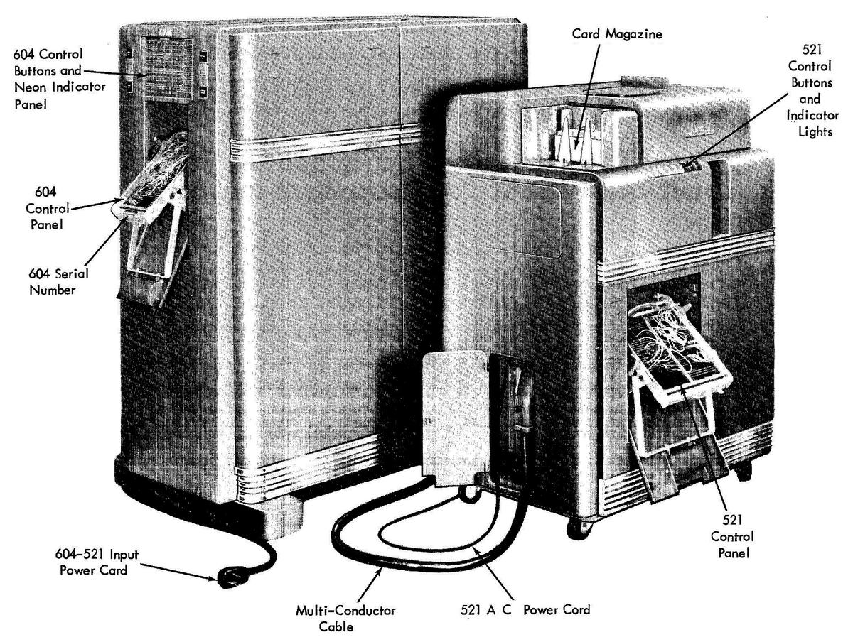
    The IBM 521 Card Reader/Punch to the right of the IBM 604 Electronic Calculating Punch.
Photo from Customer Engineering Manual of Instruction.

    The IBM 521 Card Reader/Punch to the right of the IBM 604 Electronic Calculating Punch. Photo from Customer Engineering Manual of Instruction.

    The punch cards were standard IBM 80-column cards, introduced back in 1928. The position of a hole in a column indicated the digit value for that column. For a particular task, the 80 columns would be divided into fields to hold various numbers. The 604 only supported numbers, not other alphanumeric symbols. A negative number was indicated by punching an additional hole over the units digit, using the second row from the top. (This was called an "X-punch", unrelated to the letter X.)
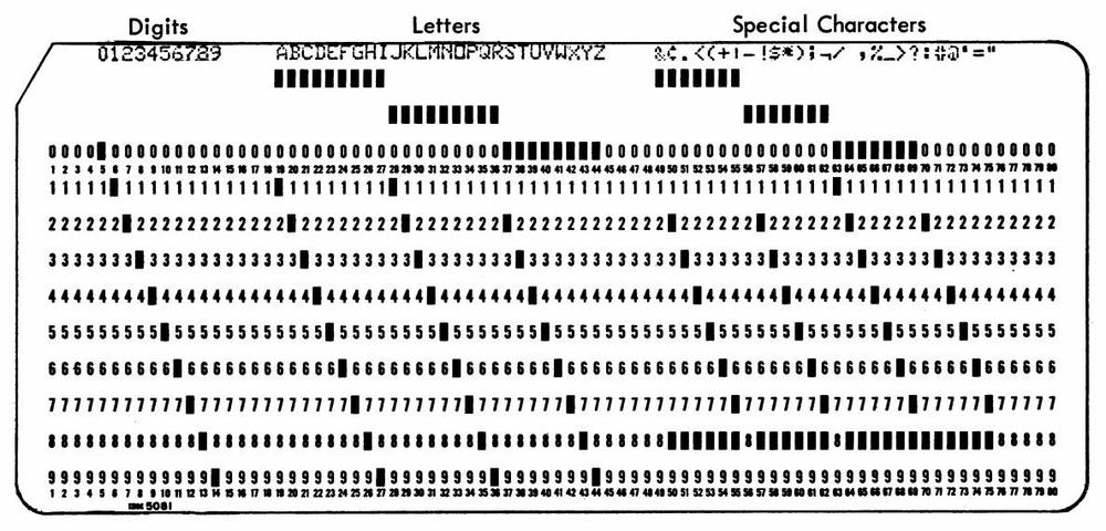
    Punch card code, from IBM 29 Card Punch Reference Manual. This code is somewhat later, with a variety of special characters.

    Punch card code, from IBM 29 Card Punch Reference Manual. This code is somewhat later, with a variety of special characters.

     ↩

  2. An interesting video showing the manufacturing and operation of the IBM 604 is here. For information on the IBM 604, see the Operating Manual. The Customer Engineering Manual of Instruction explains the 604 in detail, showing a TR-3 tube module on page 20. See IBM's Early Computers for information on the development of the 604. ↩

  3. You can think of a triode as analogous to an NPN transistor, with the grid as the base, the plate as the collector, and the cathode as the emitter. ↩

  4. The IBM 604 also used dual-triode vacuum tubes with nine pins, rather than seven, such as the type 5965. (Seven and nine pins were standard sizes for tubes.) The nine-pin tubes had separate connections for each cathode; this allowed the tubes to be used in circuits such as "cathode followers". The two filaments were in series, sharing a common "middle" pin, which is why the tube used nine pins instead of 10. ↩

  5. For a discussion of filament voltages, see Valves, 1939. This article discusses how car radios motivated the use of 6.3 volt filaments in the United States, where 6-volt car batteries were common. ↩

  6. The 2033 tube is very similar to the popular 6J6 tube, but optimized for computer circuits. The IBM 1684 tube is also very similar. The tube module that I examined was missing its tube, so I can't guarantee that the 2033 is the correct tube. ↩

  7. The standardized tube modules weren't as standardized as one might expect. For instance, the 604 used 27 different types of inverter modules in total. For a detailed discussion of the tube inverter, see IBM 604 CE Manual, pages 26-41. ↩

  8. A trigger circuit is symmetrical, so how do you define whether a trigger circuit is on or off? IBM's convention was that if the left triode was conducting, the trigger was on, while if the right triode was conducting, the trigger was off. See IBM 604 CE Manual, page 54. ↩

  9. The 604 manual includes a schematic of the TR-3 module (and other modules). Inconveniently, I didn't find this schematic until I had reverse-engineered the module; I made minor adjustments to my schematic based on this. This schematic is a bit tricky to interpret. All the resistances are in thousands of ohms (e.g. 1 is 1 KΩ), and capacitances are in "micromicrofarads" (i.e. pF). The circled numbers indicate pins of the module, while numbers in square boxes indicate voltages according to an obscure standard: 2 is +150V, and 5 is -100 V. "2-110" and "300638" are IBM part numbers. "6J" indicates that the tube is in the 6J family, where 6 indicates the heater voltage and J indicates a triode. The 604 documentation used cryptic boxes as symbols for the modules, with the arrows indicating the inputs and outputs; note that output 7 is at a lower position than output 8, indicating a lower voltage level.
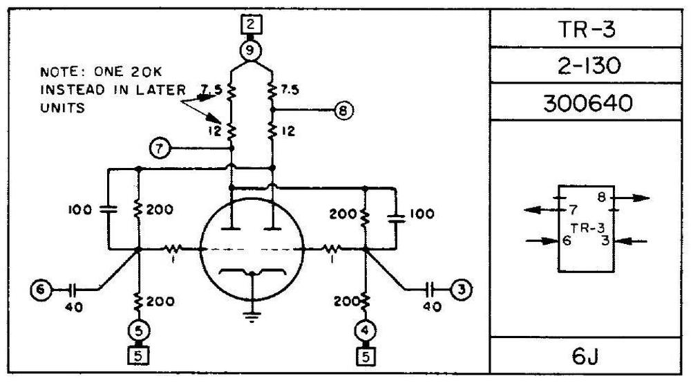
    Schematic from the CE Manual of Instruction, page 260.

    Schematic from the CE Manual of Instruction, page 260.

     ↩

  10. The two outputs from the trigger module are at different voltage levels. The idea is that a circuit could use either output, depending on which voltage level was more convenient. The asymmetrical outputs caused me great trouble, however, since I wanted to attach neon bulb indicators to show the state of both outputs. I had to carefully adjust the voltages so that the bulbs had enough voltage in the "on" state to turn on, but also a sufficiently low voltage in the "off" state to turn off. (When a neon bulb turns on, the neon gas ionizes, so it requires a significantly lower voltage to turn the bulb off.)

    The IBM 604 used neon bulbs to show the state of various circuits, both in the front panel and internally. However, unlike me, IBM used a single bulb for each trigger, either on or off, so the inconsistent voltage levels didn't cause problems. ↩

  11. The 604 used 12 different types of trigger modules, from TR-1 through TR-42. The different trigger circuits were similar, but had different component values to tune the characteristics, as well as different resistors for the output levels. A few types used resistive inputs instead of capacitively coupled inputs.

    The trigger modules were used in a variety of different ways. Briefly removing the negative bias from one side would turn that side on; this was used for reset circuits. Second, a plate could be pulled low, turning off the tube on the other side. Third, the input could be connected directly to the input, rather than going through a capacitor, with a negative voltage turning the triode off and a positive voltage turning the triode on. Other triggers used a capacitor between the plate and grid on each side to filter out noise and contact bounce. Some triggers used capacitor inputs (as in the module I described), but fed the same negative input pulse to both sides. The pulse is ignored by the triode that is on, but flips the triode that is off. The result is that the trigger switches state on each pulse—analogous to a toggle flip-flop—and divides the input pulses by two. ↩

Examining circuit boards from the Space Shuttle's I/O Processor

The Space Shuttle's five1 general-purpose computers played a critical role in each flight: controlling the engines, monitoring thousands of sensors, displaying data to the astronauts, and navigating the Shuttle. Each computer consisted of two 60-pound aluminum-alloy boxes: the box on the right is the CPU, a 32-bit processor that executed 420,000 instructions per second. These computers were designed before microprocessors became popular, so the processor was built from multiple boards crammed with simple chips and they used magnetic core memory rather than DRAM chips.

The Space Shuttle IOP and CPU (AP-101B). Photo courtesy of RR Auction.

The Space Shuttle IOP and CPU (AP-101B). Photo courtesy of RR Auction.

The box on the left is the I/O Processor (IOP): the link between the CPU and the rest of the Shuttle. It implemented the input/output capabilities for the computer, primarily 24 high-speed networks that connected the computer to the Shuttle's systems and sensors. But the IOP wasn't just a peripheral; it was a separate programmable computer, more complicated than the main CPU. The IOP had an unusual architecture: it was one of the first multi-threaded computers, implementing 25 virtual processors (with two completely different instruction sets) that ran on one physical processor.

I obtained two circuit cards from the I/O Processor,2 each a 9"×3" rectangle packed with tiny chips and other components. In IBM lingo, each card is called a "page" (remember this term). The top page is a network interface, providing four network connections, each handling 1 million bits per second. (The IOP contained six of these cards for its 24 network connections.) The bottom page held the microcode for the IOP's processors, the low-level code that defined each instruction. The rows of white-and-gold chips stored the microcode's bits in tiny metal fuses, programmed by blowing a fuse for each 1 bit. In this article, I'll explain how the I/O Processor worked, and the roles of these two pages.

Two pages from the Space Shuttle I/O Processor: the "MIA" interface page and the PROM page.

Two pages from the Space Shuttle I/O Processor: the "MIA" interface page and the PROM page.

The MIA interface page

The Space Shuttle had 28 data bus networks that linked the computers to the rest of the Shuttle, with each computer attached to 24 of the networks.3 The large number of networks provided both high performance and reliability, with at least two networks between a computer and any Shuttle system. Eight networks were assigned to flight-critical systems, with each CRT display and engine controller connected to four networks for redundancy.

The page below is one of the six network interface pages in the I/O Processor. Space Shuttle engineers loved acronyms, so this page has the cryptic name MIA for "Multiplexer Interface Adapter". (Many of the networks were connected to boxes called Multiplexer/Demultiplexers, which provided the link between the network and the diverse analog and digital components of the Space Shuttle.5) The MIA interface page is tightly packed with integrated circuits and other components. The page holds two printed-circuit boards, one on each side of the page. The boards on both sides are almost identical,4 as you can see by comparing the photo above and the photo below. (Main difference: the connector switches sides.)

The network interface page, called the MIA (Multiplex Interface Adapter).
The page has extensive rework; thin brown "bodge" wires snake around the page to
repair errors or implement updates.

The network interface page, called the MIA (Multiplex Interface Adapter). The page has extensive rework; thin brown "bodge" wires snake around the page to repair errors or implement updates.

Each board implements two network interfaces, so the page supports four networks. Each network transmits data across a pair of wires, twisted together and shielded, rather than a coaxial cable. Although the network transmits digital data, the signals transmitted across the network are physical voltages that will weaken with distance and will have distortion and noise. Thus, the interface page must convert these analog signals back to 0's and 1's.

The right half of the board holds the analog circuitry. It is dominated by a large golden module labeled "IBM", with 46 pins. This is a hybrid module, consisting of tiny components such as transistor dies, resistors, capacitors, and potentially IC dies, connected by bond wires thinner than a hair. It's not quite an integrated circuit, but a collection of individual components mounted on a ceramic wafer. Hybrid modules were popular for aerospace applications, since a board of analog components could be shrunk down to a single (expensive) module. This module contains the analog circuitry for two I/O ports: the drivers to transmit network signals along with the amplifiers and comparators to receive signals.

Various discrete components are mounted next to the hybrid module: resistors, glass capacitors6, inductors, and small square transformers. The transformers provide the coupling between the interface board and the network. As with Ethernet, transformers provide isolation between the computer and the network, filter electromagnetic interference, and match impedances, all important for reliability.7

The Manchester Mark 1; Prof. Williams is second from the left. Photo from the University of Manchester.

The Manchester Mark 1; Prof. Williams is second from the left. Photo from the University of Manchester.

A key part of the Shuttle's networking dates back to the 1940s. In 1946, Frederic Williams became head of the Electrical Engineering department at the University of Manchester. By 1949, his team had created the groundbreaking Manchester Mark 1 computer. Along the way, they invented the stored-program computer, the Williams tube—the best form of computer memory before magnetic core—and the Manchester Carry Chain, still used for addition in modern processors.

But the relevant invention is the patented Manchester encoding, a way of encoding a sequence of 0's and 1's for storage or transmission. In the Manchester encoding, each 0 bit is replaced by a "low-high" sequence and each 1 bit is replaced by a "high-low" sequence, as shown below. This idea may seem trivial, but it is used in everything from floppy disks and remote controls to Ethernet and RFID tags, earning it recognition as an IEEE Milestone.

A diagram illustrating Manchester encoding. From Prototype IOP Functional Description, p82.

A diagram illustrating Manchester encoding. From Prototype IOP Functional Description, p82.

The obvious approach—sending binary data unencoded—has two problems. First, in a long string of 0's or 1's, it is hard to tell how many bits were sent: "Was that six bits or only five?" Second, such a sequence is unbalanced, so it has a "DC component". This DC component causes problems if the signal is stored on a magnetic medium or transmitted through a transformer. The Manchester encoding solves both these problems. Since every encoded bit has a transition in the middle, it is straightforward to separate the bits. Moreover, the encoding ensures that 0's and 1's occur in equal numbers, so there is no DC component.

Because of these advantages, the Manchester encoding was selected for the data bus networks in the Space Shuttle.8 One of the key functions9 of the IOP's network interfaces is to convert between serial bits and the Manchester encoding. The digital circuitry for the interface is fairly complicated, but most of the logic is in the four large golden integrated circuits. These are custom Motorola integrated circuits: a transmit chip and a receive chip for each network port. On the transmit side, the chip converts binary data into the Manchester-encoded signals for the network. The circuitry also inserts a sync signal at the beginning of each word and adds parity. The receive chip reverses this process: detecting sync, decoding the Manchester signals, verifying the parity, and reporting any errors.

The smaller black chips are simple TTL chips, mostly shift registers. (Transistor-Transistor Logic was very popular in the 1970s, providing fast, reliable circuits.) There are twelve 4-bit shift register chips and sixteen 8-bit shift registers.10 The Shuttle's networks sent 24-bit words across the network: combining six 4-bit shift register chips produces a 24-bit shift register, which converted these 24-bit words to serial data and vice versa. The remaining chips are simple logic gates, flip-flops, buffers, and four-bit counters.

The physical structure of a page

Around 1967, IBM introduced a line of computers for avionics, called System/4 Pi.11 These systems were constructed from pages:12 two circuit boards sandwiching a metal layer that provided conduction cooling. Flat-pack integrated circuits, smaller than a fingernail, were mounted in rows13 on each circuit board, about 78 ICs on a board. The printed-circuit boards were advanced for the time, with six layers of wiring. Two jack screws at the top tightly secured the page into the system. Two 98-pin connectors connected the page to the backplane. The photo below shows a typical 4 Pi page (top), with its rows of chips.

A comparison of a standard IBM 4 Pi page with the IOP page. 4 Pi page courtesy of Eric Schlaepfer. The 4 Pi page was in a bag labeled "FSD AWACS tester?" suggesting that it was a tester from IBM's Federal Systems Division for the E-3C Airborne Warning and Control System aircraft, which used an IBM 4 Pi computer.

A comparison of a standard IBM 4 Pi page with the IOP page. 4 Pi page courtesy of Eric Schlaepfer. The 4 Pi page was in a bag labeled "FSD AWACS tester?" suggesting that it was a tester from IBM's Federal Systems Division for the E-3C Airborne Warning and Control System aircraft, which used an IBM 4 Pi computer.

An I/O processor page (above, bottom) is almost identical to a standard 4 Pi page except that it is one inch wider (9" instead of 8"), and has a 120-pin connector or two instead of 98-pin connectors.14 One inch may not seem like much, but a 9-inch page fits 100 ICs rather than 78, a significant increase. I'm surprised that IBM changed from the standard size, but I suspect that the designers couldn't fit the IOP into the available space with standard pages, forcing the change. Likewise, the multiple I/O ports may have required more connections than the smaller connectors could support.

A page has circuit boards on either side, separated by a metal plate. To allow signals to flow between the boards, a special connector is attached to the top of the page to link the two boards. This connector not only provides feed-through connections between the boards, but also provides test points, so signals can be probed while the boards are mounted in the case. The photo below shows a close-up of the feed-through connector. It has three rows of test points. The first row (red) is connected to the top board. The middle row (orange) is connected to both boards and provides the feed-throughs. The bottom row (blue) is connected to the bottom board. The upper arrows show where the connector is soldered to the board.

The test point connector on the MIA page.

The test point connector on the MIA page.

The diagram below shows the construction of the I/O Processor, with rows of pages plugged into the backplane.15 Note the 128-pin MIA I/O connector on the front of the IOP; this connects the 24 data buses (along with other signals) to other parts of the Shuttle. The arrows show how cooling air flowed through the sides of the IOP. The air did not flow over the pages. Instead, heat was transmitted by conduction through the metal plate inside each page, flowing to heat exchangers in the sides of the case. The CPU and the IOP both contained magnetic core memory (labeled "Storage Page" below); even though the memory is split between the boxes, it is treated as a unified shared memory, so programs for the CPU and the IOP can reside in memory in either physical box.

Exploded view of the IOP. From Prototype IOP Functional Description.

Exploded view of the IOP. From Prototype IOP Functional Description.

The IOP's architecture and the PROM page

The high-performance design of the I/O Processor was developed by Peter Kogge, an expert in parallel processing architectures. At the time, he was working at IBM's Federal Systems Division, where the Space Shuttle computer was developed.24 Kogge, now a professor at the University of Notre Dame, is also known for the Kogge-Stone adder, a fast circuit used in processors such as the Pentium. The I/O Processor has a very unusual architecture: although it had one physical processor, it ran 25 virtual processors with two completely different instruction sets. The virtual processors took turns, running for just one clock cycle and then letting the next processor run. The motivation behind this was to ensure that each network port got a predictable and guaranteed portion of the processor, so even if one network port was overloaded, it wouldn't affect the others. This approach, called a barrel processor16, was first used in the CDC 6600 supercomputer, the world's fastest computer from 1964 to 1969.

The I/O Processor has two types of (virtual) processors, which of course have cryptic acronyms: BCE and MSC. Each of the 24 network ports has a BCE, a Bus Control Element, which runs a small program to move data words between the network port and memory. An MSC (Master Sequence Controller) is the executive, running programs to manage the BCEs. The BCE and MSC processors run code that is stored in the computer's core memory. The instruction sets of the MSC and the BCE are completely different from each other and from the instruction set of the main CPU (which is derived from IBM's System/360 mainframes). The (executive) MSC is a 32-bit processor with the standard instructions of a normal processor—addition, logic, branches, and so forth—as well as specialized operations to configure and start BCEs.17 The instruction set of a low-level BCE is much smaller and much stranger, lacking all the basic instructions such as arithmetic and conditional branches. the instructions you'd expect from a processor. Instead, a BCE has I/O instructions such as Transmit Data, Receive Data, Load Timeout Register, Store Status, and Wait. In typical use, the CPU directs the MSC to run a program, the MSC configures the BCEs to execute a program, and the BCEs send and receive data as specified. When the BSE's operation is done, the MSC interrupts the CPU, which processes the data. Thus, the CPU can focus on the high-level algorithms without wasting cycles on network operations.

How do the MSC and BCE processors all run on one physical processor, when they have completely different instruction sets? The trick is microcode: each MSC and BCE instruction was implemented in microcode, through a sequence of 72-bit micro-instructions.18 A simple instruction might take five micro-instructions, while a complex instruction might require 60 micro-instructions. Each micro-instruction directed the action of the IOP's physical processor for one step of the MSC or BCE instruction. After each micro-instruction, the physical processor switched to the micro-instruction for the next virtual processor. The architecture of the physical processor was completely different from the MSC or the BCE: three 16-bit data paths and two ALUs (Arithmetic/Logic Units) that can operate in parallel. The physical processor had a separate register set, including a micro-instruction address register, for each virtual processor, to keep track of the state of each virtual processor.

The PROM page holds the majority of the microcode for the I/O Processor. Although three chips are mounted sideways to avoid wasting space, there is even more wasted space at the left.

The PROM page holds the majority of the microcode for the I/O Processor. Although three chips are mounted sideways to avoid wasting space, there is even more wasted space at the left.

The IOP's micro-instructions were stored in the PROM page above. In the photo above, the white chips with gold lids are fusible-link PROM (Programmable Read-Only Memory) chips.19 These unusual chips contain a tiny fuse for each bit. If the fuse is intact, the corresponding bit is a 0, while a burnt-out fuse represents a 1 bit. The chip is programmed by applying 17-volt pulses to destroy fuses one by one, literally burning the PROM. (I discussed fusible PROM chips earlier.)

Each PROM chip holds 512 words of 4 bits, so in total, this page held 1024 72-bit micro-instructions; the remaining 512 micro-instructions were in another page.20 The chips are hand-labeled with numbers, since each chip has unique programming and must be installed in the correct location. With 36 chips, you'd expect the chips to be numbered from 1 to 36. Curiously, although many of the chips are sequentially numbered, others have numbers ranging from 55 to 74 in no obvious pattern.21

Physically, the PROM page is unusual in several ways. Instead of flat-pack integrated circuits, it uses DIP (Dual-Inline Package) ICs, larger integrated circuits with two rows of vertical pins that go through the circuit board. Since this page only has one circuit board, it doesn't have the test-point feed-throughs at the top. It still has the central metal plate, but the integrated circuits sit on top of the metal plate, while the circuit board is underneath—the plate has gaps for the pins. Between the rows of chips, the central plate is the full thickness of the board.

A close-up of the PROM page, showing how the chips are mounted. The black chips are much thicker than the white chips.

A close-up of the PROM page, showing how the chips are mounted. The black chips are much thicker than the white chips.

Presumably, the fusible-link PROM chips were only available in DIP packages, rather than flat-packs. These DIP packages take up much more space than the regular flat-pack integrated circuits; this page has about a quarter the density of a regular page.22

Conclusions

The Space Shuttle's CPU and IOP were advanced when they were designed, but they rapidly became obsolete. IBM redesigned the computer, combining both the CPU and IOP into a single box called the AP-101S, which first flew in 1991 (details). The improved computer was much faster and had more memory. Moreover, combining two boxes into one saved about 300 pounds in total. The photo below shows three of the updated AP-101S computers mounted in the Shuttle's avionics bays. (The wall hides the fourth computer, and the fifth is behind the camera.) These same positions are where the I/O Processors were mounted previously, with the CPUs installed in the empty spaces to the left.

Avionics bays 1 and 2 are located in the crew cabin middeck, below the flight deck, and looking forward into the nose. The red arrows indicate the AP-101S computers. The remaining computer is in avionics bay 3A, on the aft right side of the middeck. This photo is from 2011, showing Discovery being prepared for display at the Smithsonian. Original photo courtesy of collectSpace; I've adjusted the lighting.

Avionics bays 1 and 2 are located in the crew cabin middeck, below the flight deck, and looking forward into the nose. The red arrows indicate the AP-101S computers. The remaining computer is in avionics bay 3A, on the aft right side of the middeck. This photo is from 2011, showing Discovery being prepared for display at the Smithsonian. Original photo courtesy of collectSpace; I've adjusted the lighting.

Despite the critical role of the I/O Processor in the Space Shuttle, it doesn't get the attention given to the CPU. For instance, although NASA documents describe the architecture of the IOP in detail, I couldn't find any photos of its pages.23 I hope that this article has convinced you that the architecture and the physical construction of the IOP make it an interesting system.

For updates, follow me on Bluesky (@righto.com), Mastodon (@[email protected]), or RSS. Thanks to Richard for supplying the boards. Thanks to Mike Stewart for documents on the IOP. Thanks to Robert Pearlman of collectSPACE, and RR Auction for photos.

AI statement: I didn't use AI to write this article; the em-dashes are natural (details).

Notes and references

  1. On some flights, a sixth computer was carried in a locker as a spare, providing an additional degree of reliability. If one of the five computers failed, the astronauts could connect the cables to the spare computer and it could take over for the failed one. The spare was put into use on flight STS-30 (1989) after computer #4 encountered a "data parity external storage error", indicating a hardware problem. ↩

  2. I suspected that these pages were from the I/O Processor, but it was difficult to prove this. Fortunately, Mike Stewart found a document, the Prototype Input/Output Processor Function Description, that lists the pages in each IOP slot. The MIA page has a part number on it: 6246523-3, and the PROM page has 6104848-3; these match "MIA" 6246523-1 and "Micro Store (ROM)" 6104848-1 in the document. ↩

  3. The diagram below shows how the 28 data bus networks connect the five computers at the top and various parts of the Shuttle. The networks are categorized as ground interface, mission critical, flight instrumentation, display system, mass memory, intercomputer, and flight critical.

    Data bus architecture. Click for a larger version. Adapted from Space Shuttle Avionics Systems.

    Data bus architecture. Click for a larger version. Adapted from Space Shuttle Avionics Systems.

    Why was each computer connected to 24 networks and not all 28? Each Space Shuttle computer was connected to almost all the networks, so they could run in lockstep for reliability. The exception was that each computer sent its own monitoring data to the ground station. Since this data was of no importance to the other computers, it was sent over a private network called Flight Instrumentation to the PCM (Pulse Code Modulation) box, which encoded the data for transmission to the ground. There were 23 shared networks and 5 private networks (one for each computer), so there were 28 networks in total, with 24 networks connected to a particular computer. ↩

  4. Both sides of the interface page are almost identical. However, the connector is on the left or the right side, depending on which side of the page you examine. This forced the decoupling capacitors at the very bottom to move to accommodate the connector. I also found a single integrated circuit that was different between the two sides, for some reason. ↩

  5. While many of the data bus networks are connected to a Multiplexer/Demultiplexer (MDM), this is not always the case. Networks were also connected directly to systems such as an Engine Interface Unit or a Display Electronics Unit. Moreover, the MDM was not necessarily the final step between the network and the Shuttle's sensors. The MDM held cards to support over a dozen types of input and output signals: digital, analog, on/off (discrete), and serial. However, the thousands of signals in the Shuttle were much more diverse; sensors can provide AC signals, pulses, thermocouple values, resistances, and so forth. Other boxes converted the raw sensor signals into forms that the MDM could handle; these boxes were called Dedicated Signal Conditioners (DSC). A DSC had 15 or 30 slots to hold cards to perform the necessary signal conversion. Thus, the MDMs and DSCs combined a fixed architecture with the ability to be customized for each role. ↩

  6. The glass capacitor is an interesting component, with an extremely thin layer of glass as the dielectric. Glass capacitors became popular in the 1960s for aerospace applications because of their stability and reliability (more). These capacitors were manufactured by Corning Glass Works, as indicated by the "CGW" label on the package.

    Two glass capacitors on the MIA page.

    Two glass capacitors on the MIA page.

    The capacitor is labeled with a military code. "J" indicates the Joint Army/Navy specification. "CY" indicates a glass capacitor, "4" apparently indicates axial leads, "G" indicates the temperature/voltage, "510" is the value (51×100 = 51 pF), and "G" indicates ±2% tolerance. (I don't know why one capacitor has "0F" and the other has "4G".) ↩

  7. The Space Shuttle had a second layer of transformers between the computer and the network, ensuring a faulty device didn't bring down the network. Each device (such as the IOP) was connected to the network through a tiny device called the Data Bus Coupler. This one-inch cube contains a transformer and a few resistors to match impedance. The coupler acts as a network tap, providing a short stub from the network to a device. The coupler also provides line termination if the device is removed, ensuring signal integrity. ↩

  8. The Space Shuttle's network is very similar to the U.S. military's serial network standard MIL-STD-1553. The 1553B standard is widely used in numerous military aircraft, missiles, tanks, navy systems, the Airbus A350 commercial plane, and the James Webb Space Telescope. However, since the Space Shuttle's network and the 1553 standard were both under development in the early 1970s, the two networks are not the same. The main differences are that the Shuttle uses 24-bit words instead of 16, and has 5.5”s gap between words (details). ↩

  9. The functions of the MIA are described as:

    • Transmit and receive data
    • DC isolation
    • Parallel/serial conversion
    • Serial/parallel conversion
    • Sync generation and detection
    • Manchester encode and decode
    • Parity generation and detection
    • Bit count detection
    • Provide status to BCE.

    The functional block diagram below shows the circuitry for one port of the network interface. This circuitry is replicated twice on each board; with a board on each side of the page, the page supports four networks. The dashed Transmitting and Receiving boxes correspond, I think, to the large Motorola chips, except that the "TX" and "RX" amplifiers are in the IBM hybrid module and the transformers are discrete components.

    Functional block diagram of the MIA. From Prototype IOP Functional Description, p82. Click for a larger image.

    Functional block diagram of the MIA. From Prototype IOP Functional Description, p82. Click for a larger image.

     ↩

  10. The 4-bit shift register chips are 54LS395 chips. These chips have "tri-state" outputs, allowing them to be connected to a bus. These chips probably provide the interface between the board and the rest of the IOP; the twelve chips on a board would support a 24-bit register for each port, as expected. The 8-bit shift register chips are 54LS1964 shift registers.

    I can't figure out why there are so many 8-bit shift register chips; perhaps they act as buffers. My speculation... The Prototype IOP Functional Description states that the IOP has six 28-bit 4-word registers between the 24-bit MIA shift registers and the rest of the IOP. Could the 8-bit shift register chips form these registers, even though shifting is not necessary? The document doesn't make it clear if these registers are on the MIA page or a different page. The shift-register chips provide 256 bits of storage per page, while the register file needs 112 bits, so there are way more bits than required. Moreover, the document says that the registers are structured as 7-4&4 register files for each set of four MIAs, which sounds more like 54LS170 register file chips (for instance) than shift-register chips. Possibly, the design was modified from the Prototype Functional Description, and the 8-bit shift registers provide additional buffering. ↩

  11. The 4 Pi name is a geometry joke based on IBM's wildly popular series of mainframes, the System/360. System/360 revolutionized the computer industry with the concept of one family of computers for all applications: business and scientific. The name symbolized that System/360 covered the full 360Âș of applications. The 4 Pi name extended the idea of a circle to the 3-dimensional world: 4π is the number of steradians making up a full sphere. As IBM put it, "System/4 Pi also fills a sphere—the full spectrum of military computer needs—for airborne, space, or shipboard use." ↩

  12. The earliest 4 Pi systems (the TC line) used a different style of page, but the following computers used the standard 4 Pi pages, including the Space Shuttle's AP-101B computer. However, IBM moved to much larger pages, starting with the next computer, the AP-101C in the B-1 bomber. The Space Shuttle's upgraded computer, the AP-101S, used these larger pages. For details, see my article on 4 Pi computer history. ↩

  13. The photo below shows how the flat-pack integrated circuits are mounted on the circuit board. 16 pads are allocated to each integrated circuit; 14-pin integrated circuits "waste" two pads, while larger integrated circuits break the regular pattern. Each pad is connected to a via, a plated hole through the circuit board. These vias provide connections to wiring traces on a different layer of the circuit board; some of these traces are visible in the photo. Vias also hold the leads of through-hole components. The circuit cards in IBM System/360 mainframes used a very similar style of printed-circuit board, with a regular grid of vias. This style of board is very different from the circuit boards used in most other systems, which only had holes where necessary and routed traces less regularly. IBM's style presumably made hole drilling more efficient and was easier for automatic routing, but required thin, precise traces and multi-layer circuit boards, which were not common at the time.

    IBM's technology was highly advanced compared to consumer electronics. IBM was using six-layer printed-circuit boards and surface-mount components in the 1960s, but Apple, for instance, didn't switch to surface-mount components until two decades later. Specifically, the Apple IIGS (1986) extensively used surface-mount components, but the Macintosh SE (1987) still used entirely through-hole components a year later.

    A close-up of the IOP's PROM board.

    A close-up of the IOP's PROM board.

    The photo also illustrates how some integrated circuits are labeled with Specification Control Drawing (SCD) numbers (6088731-1) while others are labeled with standard part numbers (SN54LS151). This SCD number corresponds to a standard 54S10 NAND gate. The chips both have 1974 date codes (74xx), not to be confused with 7400-series part numbers.

    The photo below shows three different types of flat-pack ICs. The first type is most common, with leads extending from the top and bottom sides, similar to a modern surface-mount integrated circuit. The second package has a golden case. It is much smaller and thinner, with leads extending from all four sides. The third package also has leads from four sides, but is somewhat larger.

    Three types of surface-mount packages.

    Three types of surface-mount packages.

     ↩

  14. The change in page size for the IOP is documented in Prototype IOC Functional Description, which says: "Standard 4 Pi Page Extended by Width Change from 8 to 9 inches, New Standard 120 Pin Connector".

    The photo below compares the 98-pin connector on a standard IBM 4 Pi page (top) with the 120-pin connector on the IOP page (bottom). The 120-pin has a narrower pin spacing (0.05") than the 98-pin connector (0.06"), allowing more pins in the same width. However, the 120-pin connector has more spacing between the rows of pins (0.150" vs. 0.100").

    The connectors on a standard IBM 4 Pi page (top) and the IOP page (bottom). The 4 Pi page is courtesy of Eric Schlaepfer. The slight waviness is just due to bent pins.

    The connectors on a standard IBM 4 Pi page (top) and the IOP page (bottom). The 4 Pi page is courtesy of Eric Schlaepfer. The slight waviness is just due to bent pins.

    Also note that both connectors have a peg on one side and a hollow cylinder on the other. These are used for keying, to make sure that a page cannot be plugged into the wrong slot. Each page type has a different combination; with a double connector, there are 16 possible combinations. ↩

  15. The exploded view shows seven MIA (interface) pages. This doesn't make sense since there are six MIA pages for the 24 network connections, as the same document lists (in Table 4-1). That table also shows one more page in total than on the exploded view. My guess is that the system was still being changed when the document was written (some entries in the table are marked TBD), resulting in inconsistencies. ↩

  16. The virtual MSC and BCE processors take turns executing on the IOP's physical processor. A 16.5 ”s time interval is split into 33 slices: each BCE gets one time slice, the MSC gets 8 time slices, and one slice is used for BCE self-tests. Thus, the MSC gets much more execution time than a low-level BCE.

    The I/O Processor's slot timer or "wheel". Adapted from Space Shuttle Systems Handbook, 8.3.

    The I/O Processor's slot timer or "wheel". Adapted from Space Shuttle Systems Handbook, 8.3.

    Each BCE and the MSC has its own register set (called local store), so the right registers are available for each slot. The physical processor is pipelined, so there are actually four slots active at any time. ↩

  17. For details on the instruction sets of the MSC and BSE processors, see Prototype IOP Functional Description, chapter 2. ↩

  18. The IOP used a micro-instruction that was 72 bits wide. A micro-instruction controlled the physical processor by specifying the data sources, data destinations, the ALU operations, and conditional branch actions. The table below shows the structure of the micro-instruction in detail. Note that a micro-instruction controls each component of the processor separately at a low level, so it is very different from a machine instruction. A micro-instruction also provides a degree of parallelism, since it specifies three operations for each step (ALU 1 operation, ALU 2 operation, and a conditional action).

    Format of a 72-bit IOP micro-instruction. From Prototype IOP Functional Description.

    Format of a 72-bit IOP micro-instruction. From Prototype IOP Functional Description.

     ↩

  19. The PROM chips are Intersil IM5624C parts. These are similar to the Signetics 82S131 and Intel 3622 parts. The front side of the page also contains nine chips labeled "D1-6605-2", probably manufactured by Harris; perhaps these are buffers. ↩

  20. The Prototype Input/Output Processor Function Description lists two pages associated with microcode: "Micro Store (ROM)" (the page that I examined), and "Micro Store Page". I assume that the second page held the 512 words that didn't fit on the first page, along with the circuitry for the microcode control logic and registers. ↩

  21. Why are the numbers on the PROM chips semi-ordered but also somewhat random? My hypothesis is that the original chips were numbered 1 through 36 in sequence, but when chips needed to be replaced for software patches, each new chip received the next number in sequence, up to 74. ↩

  22. With flat-pack ICs, an IOP board can hold up to 20 ICs per row, so 100 ICS on a board and 200 ICs on a double-sided page. With the larger DIP packages, the PROM page holds just 45 ICs. Since DIPs are taller (thicker), the page has only a single board. This shows the large density advantage of flat-pack ICs over DIP ICs.

    The density of this page is slightly better because there are a few (15) flat-pack ICs mounted on the back of the PROM board (below). The flat-pack ICs had to be mounted between the rows of DIPs to avoid the pins of the DIP ICs. Because DIPs use through-hole mounting, their pins exit the back side of the board. The large two-pin packages above and below are decoupling capacitors, filtering the power to the ICs.

    Back of the PROM page.

    Back of the PROM page.

    The back side of the board also shows that the printed-circuit board is an inch smaller than the space available; note the gap on the right. Perhaps the circuit board was designed for a standard 8-inch 4 Pi page, but then mounted on the IOP's special 9-inch page. ↩

  23. The NASA Office of Logic Design web page has a photo of a Space Shuttle board that might be from the IOP, but its source is unknown (I asked). This board is puzzling because it has the same unusual 9" form factor as the IOP pages, but it also has many differences, so it probably came from a different Shuttle system.

    A Space Shuttle board. Note the broken connector; the plastic on these vintage Burndy connections is very often broken. From Space Shuttle Computers and Avionics.

    A Space Shuttle board. Note the broken connector; the plastic on these vintage Burndy connections is very often broken. From Space Shuttle Computers and Avionics.

    The board is a dual MIA interface; it is labeled "ADPTR. INTFC. DUAL MUX", part number "A538A762-02". This part number does not appear in the IOP documentation, and has a different format from IOP part numbers. The circuitry on the board is very similar to the IOP's interface board, with hybrid modules, transformers, and analog components. Physically, the board has the same dimensions, mounting hardware, and 120-pin connector as the IOP boards. However, the board doesn't have the test point connector at the top and the ICs are arranged haphazardly, instead of in uniform rows, so it doesn't look like it was manufactured by IBM. Moreover, the number of ICs is much smaller. On the other hand, it uses the same 54LS395 4-bit shift register chips (labeled 6088913). I would think that this was a prototype board for the IOP's board, except both boards are from 1976, based on the component dates.

    My current hypothesis is that this board was the MIA network interface in a different Space Shuttle component, probably the MDM (Multiplexer/Demultiplexer); the MDM contained a "Serial MIA" board built by Singer-Kearfott. Note that the board has Singer hybrid modules; since Singer-Kearfott invented the MIA network, it makes sense that their modules would be on an interface board. Another possibility is that this board was part of the Shuttle's IMU (Inertial Measurement Unit), which was built by Singer-Kearfott. The IMU communicated with the MDM via a serial I/O line that was very similar to the MIA protocol, but had some differences.

    Singer, by the way, is the same Singer that builds sewing machines. How did they end up making advanced components for the Space Shuttle? (Not to mention nuclear missile guidance systems.) In the 1960s, Singer diversified into defense and computers; in 1968, Singer acquired Kearfott, a defense company that built inertial navigation systems. The Singer-Kearfott SKC-2000 computer was considered for the Space Shuttle, but IBM's AP-101 was selected instead. Singer-Kearfott built the Inertial Measurement Units (IMUs) for the Space Shuttle. In 1987, Singer sold its Kearfott Guidance & Navigation division to the Astronautics Corporation. Kearfott still produces guidance and navigation systems, such as the inertial navigation system for the Global Hawk UAV and the Trident II submarine-launched ballistic missile. After a 1987 takeover and two bankruptcies, Singer is back to just sewing machines, now part of the SVP Worldwide sewing machine company. ↩

  24. Bonus photo of Peter Kogge working on the I/O Processor:

     ↩

Powering up a module from the IBM 604: an electronic calculator from 1948

1948 was an interesting time for computing. For decades, businesses had used punch card equipment that added and sorted electromechanically. Now these electromechanical relays and counting wheels were being used to build room-filling general-purpose computers such as Harvard Mark I (1944) and IBM's SSEC (1948). But slow electromechanical mechanisms were already becoming obsolete. World War II had fostered the development of electronics and vacuum tubes for radio, radar, and navigation. Electronic technology was being used in massive electronic computers, such as Colossus (1943) and ENIAC (1946). The first stored-program computer, the Manchester Baby, was built in 1948.

The IBM 604 Electronic Calculating Punch behind a Type 521 Card Reader/Punch. Photo from IBM.
Note the panels in the side of the 604 and in the front of the 521 to hold plugboards.

The IBM 604 Electronic Calculating Punch behind a Type 521 Card Reader/Punch. Photo from IBM. Note the panels in the side of the 604 and in the front of the 521 to hold plugboards.

In the midst of these technological advances, IBM introduced the Electronic Calculating Punch, type 604.1 This system may seem like a step backward: it wasn't a computer, but a programmable calculator that performed a fixed set of operations.2 However, it was much smaller3 than a computer—about the size of a double refrigerator—and much cheaper: renting for $550 a month, it was affordable by businesses and universities. Since it used vacuum tubes, it was much more powerful than electromechanical equipment; it could do 60 operations in under a second, including multiplication and division. As a result, the IBM 604 became very popular, with over 5600 units produced. Moreover, IBM's experience with electronics in the 604 led to the success of its vacuum-tube computers in the 1950s.

One of the innovations of the 604 was the pluggable module, which combined a tube and its associated circuitry as shown below. The insulated handle was used to remove and install modules in the calculator. The nine pins at the bottom of the module plugged into a socket in the 604, with the sockets connected with backplane wiring. The tube was also socketed, so a bad tube could be quickly replaced. At the right, the resistors and capacitors are mounted on insulating wafers in the module.4

A thyratron tube module from the IBM 604 Electronic Calculating Punch.

A thyratron tube module from the IBM 604 Electronic Calculating Punch.

The 604 used several different types of modules. This module has a thyratron tube, a special type of tube that acts as a high-current switch. I put this module in a circuit and powered it up. The video below shows the module controlling a light bulb. The first button sends a small signal to the module (center), turning it on and illuminating the bulb. As I'll explain below, a thyratron tube stays on until its power is cut off, which I did with the second button.

Pluggable modules may seem trivial, but they were an important innovation. Previously, vacuum tube equipment was typically built from a metal chassis with tubes mounted on the top and the other components, such as resistors and capacitors, mounted underneath. IBM developed a different approach: pluggable modules, where each module held a vacuum tube along with its associated components. These patented modules were dense, since they packed components in three dimensions. Moreover, by using a small set of standardized modules, the modules could be mass-produced and the computers assembled on a production line. Maintenance and repair were simplified; modules could be swapped to find the bad module, which was replaced with a spare. These modules were so important that IBM featured them in ads for the 604. IBM used tube modules in later vacuum tube computers, using larger eight-tube modules in the high-end 700-series computers.

An ad for the IBM 604, highlighting the pluggable modules. From Time magazine, March 31, 1952, page 65. Click this image (or any other) for a larger version.

An ad for the IBM 604, highlighting the pluggable modules. From Time magazine, March 31, 1952, page 65. Click this image (or any other) for a larger version.

Vacuum tubes and the thyratron

The IBM 604 used about 1250 vacuum tubes. While vacuum tubes come in many different types, a typical type is the triode. A triode is analogous to a transistor: a small input signal is amplified to control a much larger current. In a transistor, the control signal is applied to the gate, controlling the current between the source and drain. In a triode tube, the control signal is applied to the grid, controlling the current between the cathode and the plate.

The components of a triode vacuum tube. From IBM 604 Customer Engineering manual.

The components of a triode vacuum tube. From IBM 604 Customer Engineering manual.

The diagram above shows the construction of a vacuum tube. The heater is a filament, very similar to an incandescent light bulb, that heats up the cathode to roughly 750 ÂșC. At this high temperature, the cathode emits electrons. When a large positive voltage (say, 100 volts) is put on the plate, the negatively-charged electrons are attracted. The stream of electrons from the cathode to the plate causes a current to flow through the tube. The current is controlled by the grid: if a small negative voltage is placed on the grid, it repels the negative electrons, preventing them from reaching the plate and blocking the current through the tube.

A thyratron tube is similar to a vacuum tube, except it has a tiny bit of xenon gas inside, allowing it to handle higher current.7 Like a triode, the thyratron is controlled by the grid. However, when current starts to flow through the thyratron, the xenon ionizes and the xenon plasma carries current. Unlike a vacuum tube, the grid cannot stop the flow of current. Once the gas is ionized, a thyratron tube stays on until you remove its power5 and the gas deionizes in microseconds.6

You can see this behavior in the video. When I pushed the first button, a small control signal ionized the gas, turning the tube on. The large current through the ionized gas illuminated the light bulb. The light stayed on until I briefly cut the power with the second button; the gas deionized, turning off the tube.

The thyratron tube, type 2D21.

The thyratron tube, type 2D21.

The photo above shows the thyratron tube, type 2D21, a miniature 7-pin tube.8 The plate is visible inside the tube, with the other components hidden by the plate. The dark stain at the top of the tube is the "getter", a reactive substance such as barium that absorbs impurities inside the tube.

In the 604, thyratron tubes drove relay coils and powered the electromagnets that punched holes in cards. Other IBM systems also used these thyratron tubes. For instance, the IBM 83 Card Sorter used thyratron tubes as short-term storage to keep track of which holes had been detected in a card.

Conclusion

The IBM 604 occupies an interesting position between electromechanical accounting machines and electronic computers. Although it has the speed of an electronic computer, it was still a calculator, lacking computer features such as loops, memory, and stored programs. Despite these limitations, the 604 was highly successful and led to other important IBM products.

IBM extended the 604 in 1949 so it could be programmed by punch cards in combination with plugboards; this was called the Card-Programmed Electronic Calculator. This system was still not quite a computer, but was very useful for scientific calculation at places such as Los Alamos National Labs (link). In 1953, IBM announced the successor to the 604, the IBM 650. Unlike the 604, the 650 was a programmable, general-purpose computer; it became the most popular computer of the 1950s.

Eric Schlaepfer (TubeTime) has a box of IBM 650 modules, which we hope to power up soon. For updates, follow me on Bluesky (@righto.com), Mastodon (@[email protected]), or RSS. Thanks to CuriousMarc for extensive milling work to build the socket and colorful breakout box to hold the module.

AI statement: Despite the presence of the em dash, no AI was used in the writing of this article (details).

Notes and references

  1. For information on the IBM 604, see the Operating Manual. The Customer Engineering Manual of Instruction explains the circuitry. See IBM's Early Computers for information on the development of the 604. For a detailed description of an application, see this petroleum engineering article, using the 604 to predict the profitability of an oil property. ↩

  2. The IBM 604 operated by reading numbers from a punch card, performing up to 60 operations, and punching the result onto the punch card. This was repeated for each card, processing 100 cards per minute. The IBM 604 was not a stored-program computer, so it didn't have code. Instead, the IBM 604 was programmed by plugging wires into plugboards. The plugboard below was inserted into the 604, while a second plugboard, twice as large, went in the card punch unit to control which columns of the 80-column punch card were read and punched.

    An IBM 604 plugboard. Photo from National Museum of American History, CI.328576. (Click for a larger image.)

    An IBM 604 plugboard. Photo from National Museum of American History, CI.328576. (Click for a larger image.)

    Looking at the plugboard above, the column on the left with the heading "PROGRAM" had a row for each programming step. A wire from that row was connected to the function to be performed on that step. The system supported conditionals: the operation that was performed on a step could be changed or skipped with the calculator selectors ("CALC. SEL.") on the right. (A selector was a relay that could send a signal along one of two paths (Normal or Transfer) based on a Control input.) For more information on the plugboards, see the Operator's Manual. ↩

  3. The IBM 604 weighed 1310 pounds, while the attached 521 Card Reader/Punch weighed 670 pounds. The system used 5.5 KW of power. (Vacuum tubes are power-hungry; the module that I used required 3.75 watts for the heater alone.) ↩

  4. I reverse-engineered the MS-7A thyratron module to create the schematic below. Black pin numbers are module pins (1-9), while red pin numbers are tube pins (1-7).

    Schematic of the IBM MS-7A module, reverse-engineered.

    Schematic of the IBM MS-7A module, reverse-engineered.

    For my experiment, I powered the module with about 100 volts on the plate (pin 5). I used pin 3 of the module for the input, using about 8 volts to trigger the thyratron. Pin 4 is the output, pulled high when the thyratron fires. I connected the light bulb between pin 4 and ground (pin 6). I ignored pins 7, 8, and 9. ↩

  5. One disadvantage of a thyratron is that you need to remove its power to turn it off. In the 604, a mechanical cam in the card reader/punch activated a microswitch to turn off the power (details. Since the card reader/punch used cams on a rotating shaft for its timings, one more cam wasn't an inconvenience. ↩

  6. The behavior of a thyratron is very similar to the silicon-controlled rectifier (SCR). This semiconductor device is also called a thyristor, short for thyratron transistor. ↩

  7. The xenon pressure in the thyratron tube is very small, just .05 Torr, less than 1/10,000 of atmospheric pressure (source). Vacuum tubes, in comparison, have a vacuum that is orders of magnitude higher, around 10-6 Torr.

    Some high-power thyratron tubes use mercury vapor, such as the ones inside a 1940s power supply that we examined. These tubes give off a blue glow when active. The xenon tube, in comparison, didn't emit any light that I could see, apart from the orange glow from the filament. ↩

  8. The pinout for the 2D21 thyratron tube is shown below, and the datasheet is here. Thyratrons use the same symbols as vacuum tubes, except the large black dot indicates the presence of gas in the tube.

    Symbol for the 2D21 thyratron tube. From IBM 604 Customer Engineering manual.

    Symbol for the 2D21 thyratron tube. From IBM 604 Customer Engineering manual.

    As the symbol shows, the 2D21 tube has two grids, so it is technically a tetrode (four active elements). The second grid improves performance by screening the control grid from the cathode and the plate, reducing capacitance. (See Thyratrons for modern industry.) For my experiment, I ignored the screen grid. (The 604 also used some pentagrid tubes with a whopping five grids: two control grids, two screen grids, and a suppressor grid.) ↩