This post gives detailed background to my PyData Global talk, “GPU-Accelerated Zarr” (slides, video). It deliberately gets into the weeds, but I will try to provide some background for people who are new to Zarr, GPUs, or both.
The first takeaway is that zarr-python natively supports
NVIDIA GPUs. With a one-line zarr.config.enable_gpu() you can configure zarr
to return CuPy arrays, which reside on your GPU:
>>> import zarr
>>> zarr.config.enable_gpu()
>>> z = zarr.open_array("path/to/store.zarr", mode="r")
>>> type(z[:])
cupy.ndarray
The second takeaway, and the main focus of this post, is that that simple one-liner leaves performance on the table. It depends a bit on your workload, but I’d claim that Zarr’s data loading pipeline shouldn’t ever be the bottleneck. Achieving maximum throughput today requires some care to ensure that the system’s resources are used efficiently. I’m hopeful that we can improve the libraries to do the right thing in more situations.
This post pairs nicely with Earthmover’s I/O-Maxing Tensors in the Cloud post, which showed that network and object storage service (e.g. S3) also shouldn’t be a bottleneck in most workloads. Ideally, your actual computation is where the majority of time is spent, and the I/O pipeline just gets out of your way.
Some background
I imagine that some people reading this have experience with Zarr but not GPUs, or vice versa. Feel free to skip the sections you’re familiar with, and meet up with us at the Speed of Light section.
Zarr Background for GPU People
Zarr is many things, but today we’ll focus on Zarr as the storage
format for n-dimensional arrays. Instead of tabular data, which you might store
in a columnar format like Apache Parquet, you’re working with data that fits
things like xarray’s data model: everything is an n-dimensional array with
metadata. For example, 3-d array measuring forecasts for a temperature field
with dimensions (x, y, time).
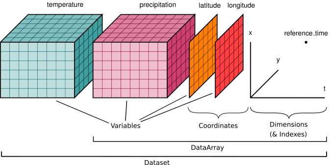
Zarr is commonly used in many domains including microscopy, genomics, remote sensing, and climate / weather modeling. It works well with both local file systems and remote cloud object storage. High-level libraries like xarray can use zarr as a storage format:
# https://tutorial.xarray.dev/intermediate/remote_data/cmip6-cloud.html
>>> ds = xr.open_zarr(
...     "gs://cmip6/CMIP6/ScenarioMIP/NOAA-GFDL/...",
...     consolidated=True,
... )
>>> zos_2015jan = ds.zos.sel(time="2015-01-16")
>>> zos_2100dec = ds.zos.sel(time="2100-12-16")
>>> sealevelchange = zos_2100dec - zos_2015jan
>>> sealevelchange.plot.imshow()
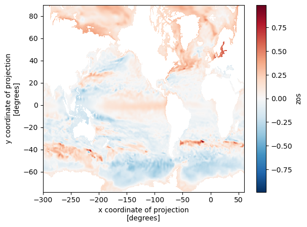
xarray knows how to translate the high-level slicing like time="2015-01-16" to
the lower level slicing of a Zarr array, and Zarr knows how to translate
positional slices in the large n-dimensional array to files / objects in
storage. This diagram shows the structure of a Zarr store:
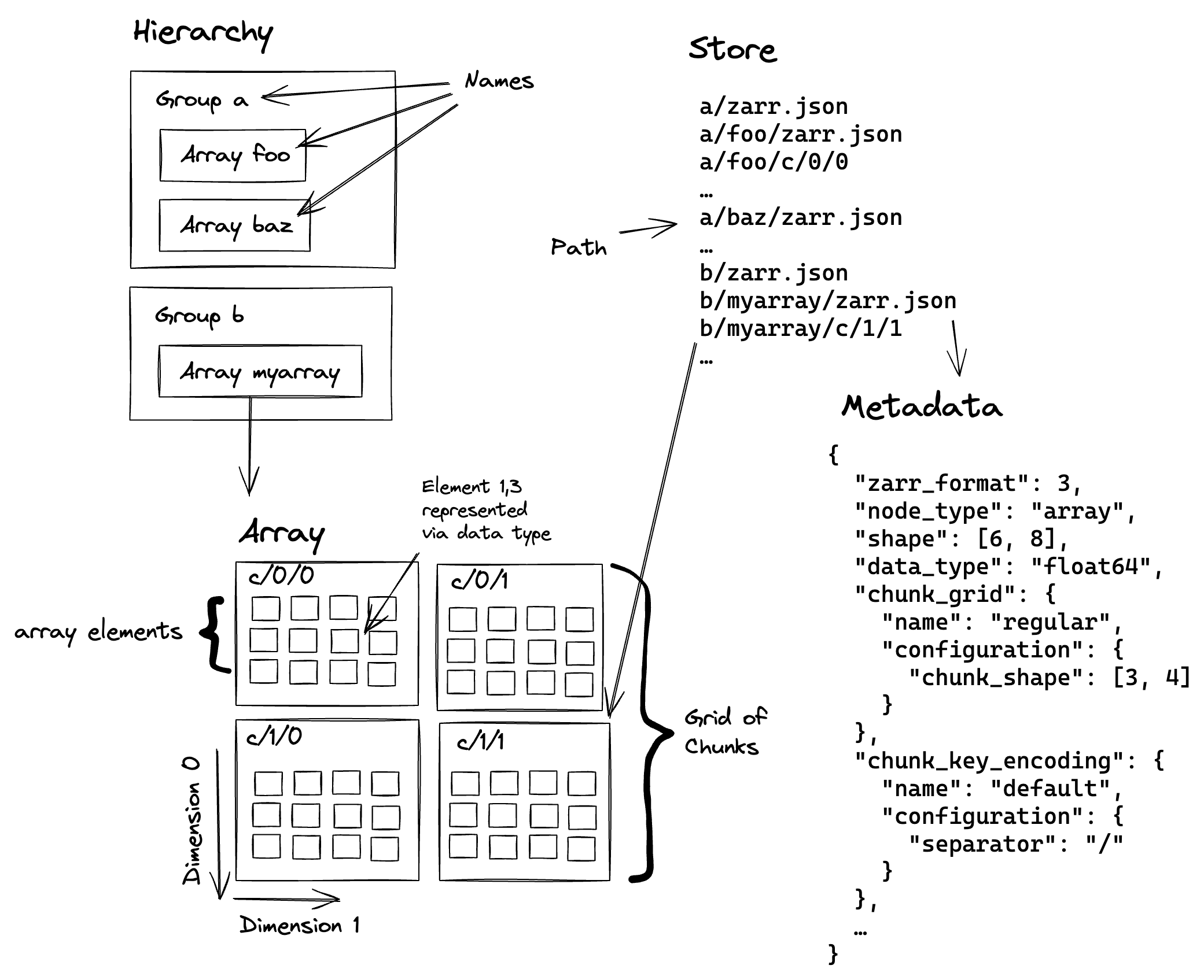
The large logical array is split into one or more chunks along one or more dimensions. The chunks are then compressed and stored to disk, which lowers storage costs and can improve read and write performance (it might be faster to read fewer bytes, even if you have to spend time decompressing them).
Zarr’s sharding codec is especially important for GPUs. This makes it possible to store many chunks in the same file (a file on disk, or an object in object storage). We call the collection of chunks a shard, and the shard is what’s actually written to disk.
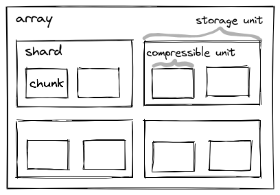
Multiple chunks are (independently) compressed, concatenated, and stored into the same file / object. We’ll discuss this more when we talk about performance, but the key thing sharding provides is amortizing some constant costs (opening a file, checking its length, etc.) over many chunks, which can be operated on in parallel (which is great news for GPUs).
For now, just note that we’ll be dealing with various levels of Zarr’s hierarchy:
- Arrays: the logical n-dimensional array
- Shards: the file on disk / object in object storage, which contains many chunks concatenated together
- Chunks: the smallest unit we can read (since it must be decompressed to interpret the bytes correctly)
GPU Background for Zarr People
GPUs are massively parallel processors: they excel when you can apply the same problem to a big batch of data. This works well for video games, ML / AI workloads, and data science / data analysis applications.
(NVIDIA) GPUs execute “kernels”, which are essentially functions that run on GPU data. Today, we won’t be discussing how to author a compute kernel. We’ll be using existing kernels (from libraries like nvcomp, CuPy, and CCCL). Instead, we’ll be worried about higher-level things like memory allocations, data movement, and concurrency
Many (though not all) GPU architectures have dedicated GPU memory. This is separate from the regular main memory of your machine (you’ll hear the term “device” to refer to GPUs, and “host” to refer to the host operating system / machine, where your program is running).
While device memory tends to be relatively fast compared to host memory (for example, it might have >3.3 TB/s from the GPU’s memory to its compute cores), it’s moving data between host and device memory is relatively slow (perhaps just 128 GB/s over PCIe). It also tends to be relatively small (an NVIDIA H100 has 80-94GB of GPU memory; newer generations have more, but still GPU memory is precious when processing large datasets). All this means we need to be careful with memory, both how we allocate and deallocate memory and how we move data between the host and device.
In GPU programming, keeping the GPU busy is necessary (but not sufficient!) to achieve good performance. We’ll use GPU utilization, the percent of time (over some window) when the GPU was busy executing some kernel, as a rough measure of how well we’re doing.
One way to achieve high GPU utilization is to queue up work for the GPU to do. The GPU is a device, a coprocessor, onto which your host program offloads work. As much as possible, we’ll have our Python program just do orchestration, leaving the heavy computation to the GPU. Doing this well requires your host program to not slow down the (very fast) GPU.
In some sense, you want your Python program to be “ahead” of the GPU. If you wait to submit your next computation until some data is ready on the GPU, or some previous computation is completed, you’ll inevitably have some time gap when your GPU is idle. Sometimes this is inevitable, but with a bit of care we’ll be able to make our Zarr example perform well.
My Cloud Native Geospatial Conference post touched on this under Pipelining. This program waits to schedule the computation until the CPU is done reading the data, and so doesn’t achieve high throughput:

This second program queues up plenty of work to do, and so achieves higher throughput:

For this example, we’ll use a single threaded program with multiple CUDA Streams to achieve good pipelining. CUDA streams are a way to express a sequence (a stream, if you will) of computations that must happen in order. But, crucially, you can have multiple streams active at the same time. This is nice because it frees you from having to worry too much about exactly how to schedule work on the GPU. For example, one stream of computation might heavily use the memory subsystem (to transfer data from the host to device, for example) while another stream might be using the compute cores. But you don’t have to worry about timing things so that the memory-intensive operation runs at the same time as the compute-intensive operation.
In pseudocode:
a0 = read_chunk("path/to/a", stream=stream_a)
b0 = read_chunk("path/to/b", stream=stream_b)

a1 = transform(a0, stream=stream_a)
b1 = transform(b0, stream=stream_b)
read_chunk might exercise the memory system to transfer data from the host to
the device, while transform might really hammer the compute cores.
All you need to do is “just” correctly express the relationships between the different parts of your computation (not always easy!). The GPU will take care of running things concurrently where possible.
One subtle point here: these APIs are typically non-blocking in your host
Python (or C/C++/whatever) program. read_chunk makes some CUDA API calls
internally to kick off the host to device transfer, but it doesn’t wait for that
transfer to complete. This is good, since we want our host program to be well
ahead of the GPU; we want to go to the next line and feed the GPU more work to
do.
If we actually poked the memory address where the data’s supposed to be it might
be junk. We just don’t know. If we really need to wait for some data /
computation to be completed, we can call stream.synchronize(), which forces
the host program to wait until all the computations on that stream are done.
But ideally, you don’t need that. For the typical case of launching some
CUDA kernel some some data, synchronization is unnecessary. You only need
to ensure that the computation happens on the same CUDA stream as the data
loading (like in our pseudocode example, launching each transform on
the appropriate stream), and you’re good to go.
CUDA streams do take some getting used to. You can make analogies to thread programming and to async / await, but that only gets you so far. At the end of the day they’re an extremely useful tool to have in your toolkit.
Speed of Light
When analyzing performance, it can be helpful to perform a simple “speed-of-light” analysis: given the constraints of my system, what performance (throughput, latency, whatever metric you care about) should I expect to achieve? This can combine abstract things (like a performance model for how your system operates) with practical things (what’s the sequential read throughput of my disk? What’s the clock cycle of my CPU?).
Many Zarr workloads involve (at least) three stages:
Reading bytes from storage (local disk or remote object storage). Your disk (for local storage) or NIC / remote storage service (for remote storage) has some throughput, which you should aim to saturate. Which bytes you need to read will be dictated in part by your application. Zarr supports reading subsets of data (with the chunk being the smallest decompressable unit). Ideally, your chunking should align with your access pattern.
Decompressing bytes with the Codec Pipeline. Different codecs have different throughput targets, and these can depend heavily on the data, chunk size, and hardware. We’re using the default Zstd codec in this example.
Your actual computation. This should ideally be the bottleneck: it’s the whole reason you’re loading all this data after all.
And if you are using a GPU, at some point you need to get the bytes from host to device memory1.
Finally, you might need to store your result. If your computation reduces the data this might be negligible. But if you’re outputting large n-dimensional arrays this can be as or more expensive than the reading.
In this case, we don’t really care about what the computation is; just something that uses the data and takes a bit of time. We’ll do a bunch of matrix multiplications because they’re pretty computationally expensive and they’re well suited to GPUs.
Notably, we won’t do any kind computation that involves data from multiple shards. They’re completely independent in this example, which makes parallelizing at the shard level much simpler.
Example Workload
This workload operates on a 1-D float32 array with the following properties:
| Level | Shape | Size (MB) | Count per parent |
|---|---|---|---|
| Chunk | (256_000,) | 1.024 | 400 chunks / shard |
| Shard | (102_400_000,) | 409.6 | 8 shards / array |
| Array | (819_200_000,) | 3,276.8 | - |
Each chunk is Zstd compressed, and the shards take about 77.5 MB on disk giving a compression ratio of about 5.3.
The fact that the array is 1-D isn’t too relevant here: zarr supports n-dimension arrays with chunking along any dimension. It does ensure that one optimization is always available when decoding bytes, because the chunks are always contiguous subsets of the shards. We’ll talk about this in detail in the Decode bytes section.
Our workload will read the data, transfer it to the GPU (if using the GPU) and perform a bunch of matrix multiplications.
Performance Summary
This example workload has been fine-tuned to make the GPU look good, and I’ve done zero tuning / optimization of the CPU implementation. Any comparisons with CPU libraries are essentially bunk, but it’s a natural question so I’ll report them anyway.
The top level summary will compare three implementations:
- zarr-python: Uses vanilla zarr-python for I/O and decoding, and NumPy for the computation.
- zarr-python GPU: Uses zarr-python’s built-in GPU support to return CuPy arrays, so the GPU is used for computation. At the moment, this still uses Numcodecs to decompress the data, which runs on the CPU. After decompression, the data is moved to the GPU for the matrix multiplication.
- Custom GPU: My custom implementation of I/O and decoding with CuPy for the computation.
| Implementation | Duration (ms) |
|---|---|
| Zarr / NumPy | 19,892 |
| Zarr / CuPy | 3,407 |
| Custom / CuPy | 478 |
You can find the code for these in my CUDA Stream Samples repository.
Please don’t take the absolute numbers, or even the relative numbers too seriously. I’ve spent zero time optimizing the Zarr/NumPy and Zarr/CuPy implementations. The important thing to take away here is that we have plenty of room for improvement. My Custom I/O pipeline just gradually removed bottlenecks as they came up, some of which apply to zarr-python’s CPU implementation as well. Follow https://github.com/zarr-developers/zarr-python/issues/2904 if you’re interested in developments.
The remainder of the post will describe, in some detail, what makes the custom implementation so fast.
Performance optimizations
Once you have the basics down (using the right data structures / algorithm, removing the most egregious overheads), speeding up a problem often involves parallelization. And you very often have multiple levels of parallelization available. Picking the right level is absolutely a skill that requires some general knowledge about performance and specific details for your problem.
In this case, we’ll operate at the shard level. This will be the maximum amount of data we need to hold in memory at any point in time (though the problem is small enough that we can operate on all the shards at the same time).
We’ll use a few techniques to get good performance in our pipeline:
- No (large) memory allocations on the critical path.
This applies to both host and device memory allocations. We’ll achieve this by preallocating all the arrays we need to process the shard. Whether or not this should be considered cheating or not is a bit debatable and a bit workload dependent. I’d argue that the most advanced, performance-sensitive workloads will process large amounts of data and so can preallocate a pool of buffers and reuse them across their unit of parallelization (shards in our case).
Regardless, if we’re doing large memory allocations after we’ve started processing a shard (either host or device allocations for the final array or for intermediates) then these allocations can quickly become the bottleneck. Pre-allocation (and reuse across shards) is an important optimization if it’s available.
- Use pinned (page-locked) memory for host buffers
Using pinned memory makes the host to device transfers much faster. More on that later.
- Use CUDA streams to overlap I/O and Computation
Our workload has a regular pattern of “read, transfer, decode, compute” on each shard. Because these exercise different parts of the GPU (transfer uses the memory subsystem, decode and compute launch kernels that run on the GPU’s cores), we can run them concurrently.
We’ll assign a CUDA stream per shard. We’ll be very careful to avoid stream / device synchronizations so that our host program schedules all the work to be done.
Throughout this, we’ll use nvtx to annotate certain ranges of code. This will make reading the Nsight Systems report easier.
Here’s a screenshot of an nsys profile, with a few important bits highlighted (open the file for a full-sized screenshot):
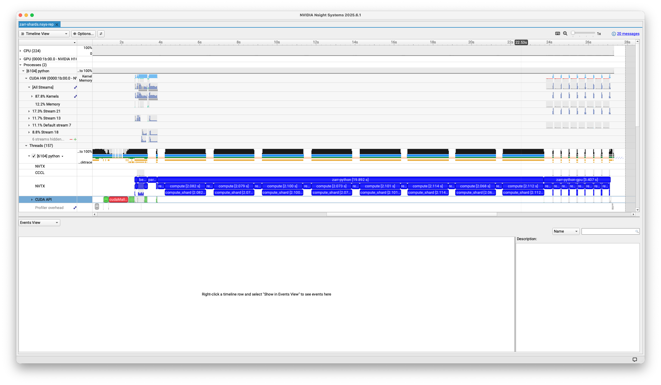
- Under Processes > Threads > python, you see the traces for our host program,
in this case a Python program. This will include our nvtx annotations
(
read::disk,read::transfer,read::decode, etc.) and calls to the CUDA API (e.g.cudaMemcpyAsync). These calls measure the time spent by the CPU / host program, not the GPU.
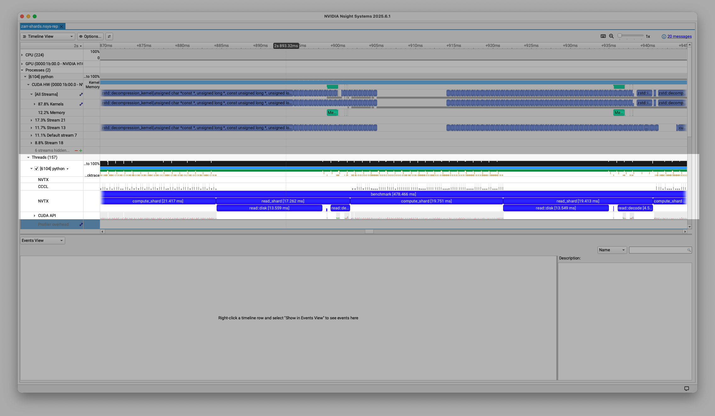
- Under Processes > CUDA HW, you’ll see the corresponding traces for GPU operations. This shows CUDA kernels (functions that run on the GPU) in light blue and memory operations (like host to device transfers) in teal.
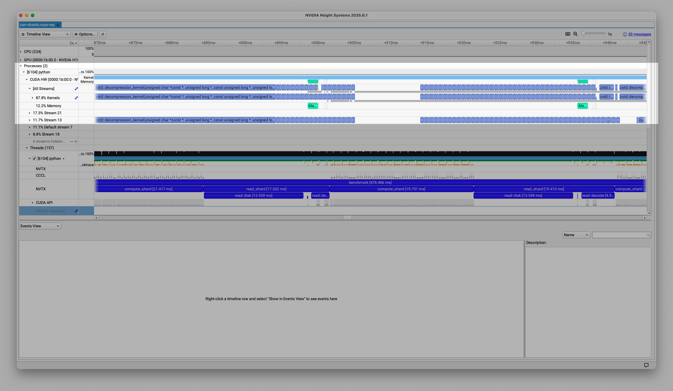
You can download the full nsight report here and open it locally with NVIDIA Nsight Systems.
This table summarizes roughly where we spend our time on the GPU per shard (very rough, and there’s some variation across shards, especially as we start overlapping operations with CUDA streams).
| Stage | Duration (ms) | Raw Throughput (GB/s) | Effective Throughput (GB/s) |
|---|---|---|---|
| Read | 13.6 | 5.7 | 30.1 |
| Transfer | 1.5 | 51.7 | 273 |
| Decode | 45 | 1.7 | 9.1 |
| Compute | 150 | 2.7 | 2.7 |
Raw throughput measures the actual number of bytes processed per time unit,
which is the compressed size for reading, transferring, and decoding.
“Effective Throughput” uses the uncompressed number of bytes for each stage.
After decompression the actual number of bytes processed equals the uncompressed
bytes, so Compute’s raw throughput is equal to its effective throughput.
Read bytes
First, we need to load the data. In my example, I’m just using files on a local disk, though you could use remote object storage and still perform well. We’ll parallelize things at the shard level (i.e. we’re assuming that the entirety of the shard fits in GPU memory).
path = array.store_path.store.root / array.store_path.path / key

with open(path, "rb") as f, nvtx.annotate("read::disk"):
    f.readinto(host_buffer)
On my system, it takes about 13.6 ms to read the 77.5 MB, for a throughput of about 5.7 GB/s from disk (the OS probably had at least some of the pages cached). The effective throughput (uncompressed size over duration) is about 30.1 GB/s. I’ll note that I haven’t spent much effort optimizing this section.
Note that we use readinto to read the data from disk directly into the
pre-allocated host buffer: we don’t want any (large) memory allocations on the
critical path. Also, we’re using pinned memory (AKA page-locked
memory) for the host buffers. This prevents the operating system from paging the
buffers, which lets the GPU directly access that memory when copying it, no
intermediate buffers required.
And it’s worth emphasizing: this I/O is happening on the host Python program, and it is blocking. As we’ll see later, time spent doing stuff in Python is time not spent scheduling work on the GPU. We’ll need to ensure that the GPU is fed sufficient work, so let’s keep our eye on this section.
The profile report for this section is pretty boring:

Note what the GPU is doing right now: nothing! There aren’t any CUDA HW
annotations visible above the initial read::disk. At least for the very first
shard we read, the GPU is necessarily idle. But as we’ll discuss shortly,
subsequent shards are able to overlap disk I/O with CUDA operations.
This screenshot shows the profile for the second shard:
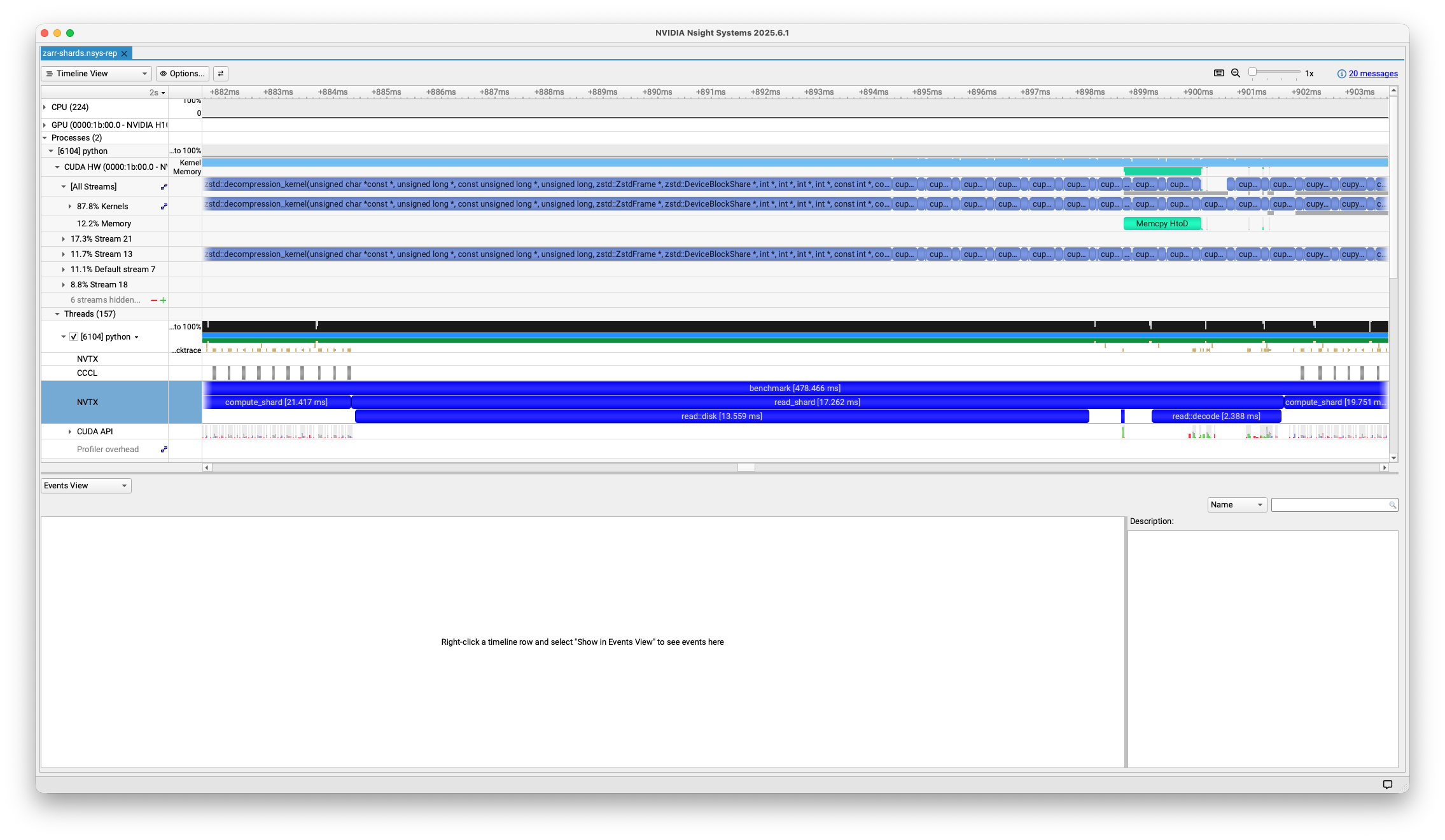
Now the GPU is busy with some other operations (decoding the chunks from the
first shard in this case, which are directly above the read::decode happening
on the host at that time). This is partly why I didn’t bother with parallelizing
the disk I/O: only one thing can be the bottleneck, and right now we’re able to
load data from disk quickly enough.
Transfer bytes
After we’ve read the bytes into memory, we schedule the host to device transfer:
with nvtx.annotate("read::transfer"), stream:
    # device_buffer is a pre-allocated cupy.ndarray
    device_buffer.set(
        host_buffer[:-index_offset].view(device_buffer.dtype), stream=stream
    )
This is where our earlier discussion on blocking vs. non-blocking APIs comes
in handy. The device_buffer.set call is not blocking, which is why it
takes only ~60 μs on the host. It only makes the CUDA API call to set up
the transfer and then immediately returns back to the Python program (to
close our context managers and then continue to the next line in our program).
The actual memory copy (which is running on the device) takes about 1.5 ms for a throughput of about 52 GB/s (this is still compressed data, so the effective throughput is even higher). Here’s the same profile I showed earlier, but now you’ll understand the context around what happens on the host (the CUDA API call to do something) and device.
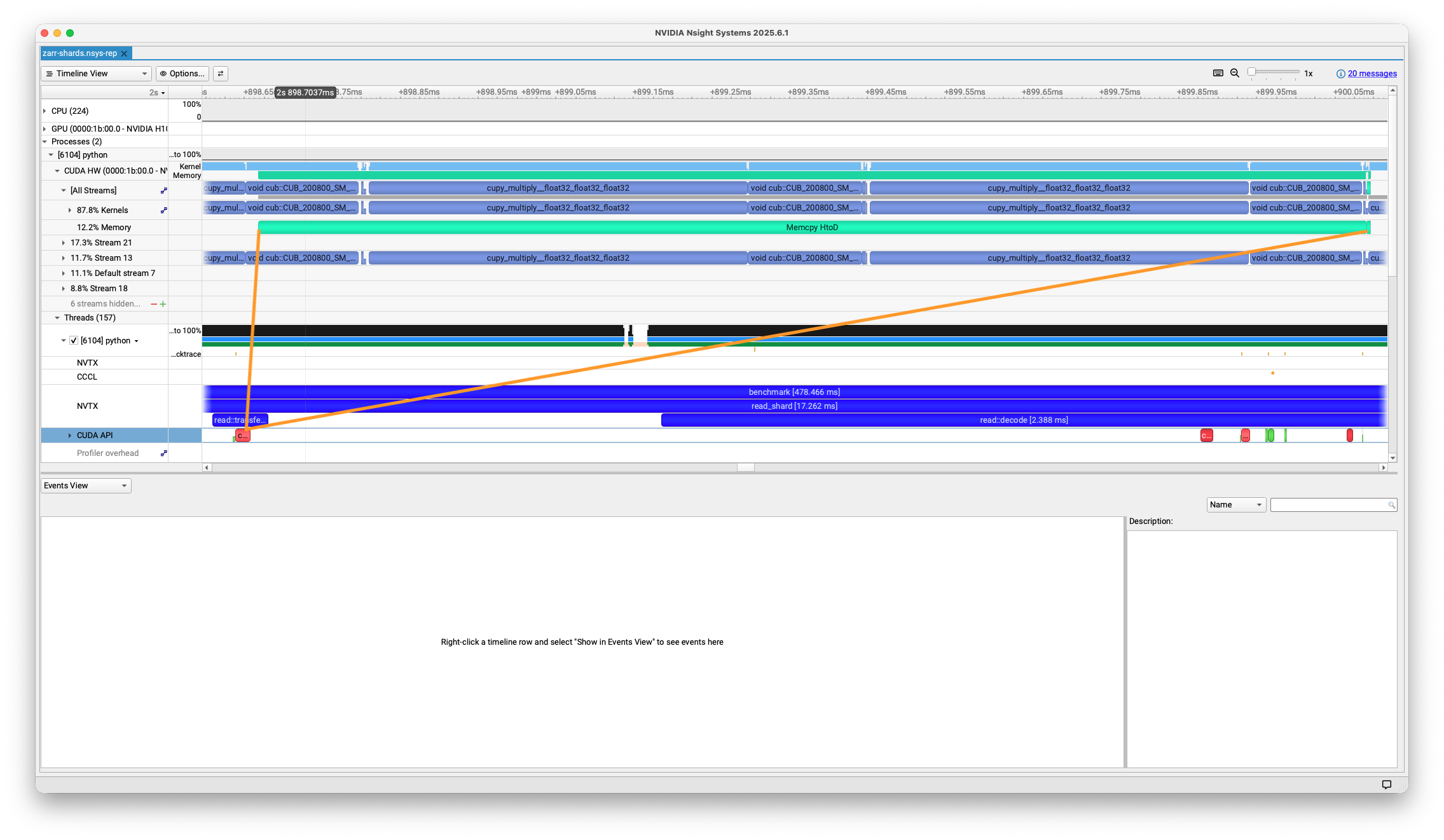
I’ve added the orange lines connecting the fast cudaMemcpyAsync on the host to
the (not quite as fast) Memcpy HtoD (host to device) running on the device.
And if you look closely, you’ll see that just above that Memcpy HtoD in teal,
we’re executing a compute kernel (in light-blue). We’ll get to that in a bit,
but this show that we’re overlapping Host-to-Device transfers with compute
kernels.
Decode bytes
At this point we have (or will have, eventually) the Zstd compressed bytes in GPU memory. You might think that “decompressing a stream of bytes” doesn’t mesh well with “GPUs as massively parallel processors”. And you’d be (partially) right! We can’t really parallelize decoding within a single chunk, but we can decode all the chunks in a shard in parallel. My colleague Akshay has a nice overview of how the GPU can be used to decode many buffers in parallel.
I have no idea how to implement a Zstd decompressor, but fortunately we don’t have to. The nvCOMP library implements a bunch of GPU-accelerated compression and decompression routines, including Zstd. It provides C, C++, and Python APIs. A quick note: this example is using a custom wrapper around nvcomp’s C API. This works around a couple issues with nvcomp’s Python bindings.
- At the moment, accessing an attribute on the decompressed array returned by nvcomp causes a “stream synchronization”. This forces essentially blocks the host program from progressing until the GPU has caught up, which we’d like to avoid. We need to issue compute instructions still, and we’d ideally move on to the next shard!
- We’d like full control over all the memory allocations, including the ability to preallocate the output buffers that the arrays should be decompressed into. This is possible with the C API, but not (yet) the Python API.
My custom wrapper is not at all robust, well designed, etc. It’s just enough to work for this demo. Don’t use it! Use the official Python bindings, and reach out to me or the nvcomp team if you run into any issues. But here’s the basic idea in code:
zstd_codec = ZstdCodec(stream=stream)
# get a list of arrays, each of which is a view into the original device buffer
# `device_buffer` is stream-ordered on `stream`,
# so `device_arrays` are all stream-ordered on `stream`
device_arrays = [
    device_buffer[offset : offset + size] for offset, size in index
]
with nvtx.annotate("read::decode"):
    zstd_codec.decode_batch(device_arrays, out=out_chunks)

# and now `out` is stream-ordered on `stream`
The zstd_codec.decode_batch call takes about 2.4 ms on my machine. Again
this just schedules the decompression call.
The actual decompression takes about 25-45 ms, for a throughput of about roughly 1.7 GB/s.
Again, we’ve pre-allocated the out ndarray, however this is not always
possible. Zarr allows chunking over arbitrary dimensions, but we’ve assumed
that the chunks are contiguous slices of the output array2. If
your chunks aren’t contiguous slices of the output array, you’ll need to
decode into an intermediate buffer and then perform some memory copies
into the output buffer.
Anyway, all this is to say that decompression isn’t our bottleneck. And this is despite decompression competing for GPU cores with the computation. The newer NVIDIA Blackwell Architecture includes a dedicated Decompression Engine which improves the decompression throughput even more.
And for those curious, a brief experiment without compression is about twice as slow on the GPU as the version with compression, though I didn’t investigate it deeply.
Computation
This example is primarily focused on the data loading portion of a Zarr workload, so the computation is secondary. I just threw in a bunch of matrix multiplications / reductions (which GPUs tend to do quickly).
But while the specific computation is unimportant, there are some characteristics to consider about your computation, it should take some non-negligible amount of time, such it’s worthwhile moving the data from the host to the device for the computation (and moving the result back to the host).
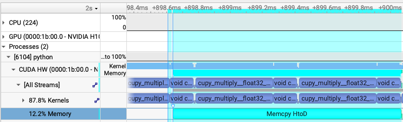
The key thing we care about here is overlapping host to device copies with compute, so that the GPU isn’t sitting around waiting for data. Note how the teal Host to Device Copy is running at the same time as the matrix multiplication from the previous shard:
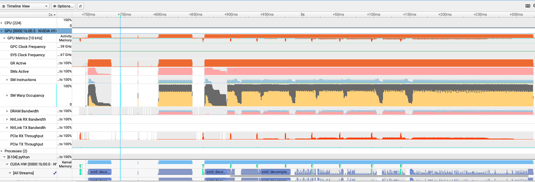
And at this point, you can start analyzing GPU metrics if you still need to squeeze additional performance out of your pipeline.
But I think that’s enough for now.
Summary
One takeaway here is that GPUs are fast, which, sure. A slightly more interesting takeaway is that GPUs can be extremely fast, but achieving that takes some care.
In this workload my custom pipeline achieved high throughput by
- Being very careful with memory allocations and data movement.
- Using pinned host memory to speed up the one host to device transfer per shard
- Use nvcomp and Zarr shards to parallelize decoding many chunks on the GPU
- Use CUDA streams to express our workloads’ shard-level parallelism, so that we can overlap host I/O, host-to-device copies, kernel launches and kernel execution.
I’m hopeful that we can optimize the codec pipeline and memory handling in zarr-python to close the gap between what it provides and my custom, hand-optimized implementation (0.5s). But doing that in a general purpose library will require even more thought and care than my hacky implementation.
If you’ve made it this far, congrats. Reach out if you have any feedback, either directly or on the Zarr discussions board.
NVIDIA does have GPU Direct Storage which offers a way to read directly from storage to the device, bypassing the host (OS and memory system) entirely. I haven’t tried using that yet. ↩︎
Explaining that optimization in more detail. We need the chunks to be contiguous in the shard. Consider this shard, with the letters indicating the chunks:
| a a a a |
| b b b b |
| c c c c |
| d d d d |
In C-contiguous order, that can be stored as:
| a a a a b b b b c c c c d d d d|i.e. all of the
a’s are together in a contiguous chunk. That means we can tell nvcomp to write its output at this memory address and it’ll work out fine. Likewise forb, just offset by some amount, and so on for the other chunks.However, this chunking is not amenable to this optimization because the chunks aren’t contiguous in the shard:
| a a b b |
| a a b b |
| c c d d |
| c c d d |
Maybe someone smarter than me could pull off something with stride tricks. But for now, note that the ability to preallocate the output array might not always be an option.
That’s not necessarily a deal-killer: you’ll just need a temporary buffer for the decompressed output and an extra memcpy per chunk into the output shard. ↩︎