Bayesian Additive Regression Trees (BART)

Posted on March 20, 2020 by kjytay

Bayesian Additive Regression Trees (BART), proposed by Chipman et al. (2010) (Reference 1), is a Bayesian “sum-of-trees” model where we use the sum of trees to model or approximate the target function $f(x) = \mathbb{E}[Y \mid x]$ , where $Y$ is the response of interest and $x$ represents the covariates that we are using to predict $Y$ . (If there are $p$ covariates, then $x$ is a $p$ -dimensional vector.) It is inspired by ensemble methods such as boosting, where a meta algorithm combines a large number of “weak learners”/”weak predictors” to get a much more accurate prediction.

As a Bayesian method, all we have to do is to specify the prior distribution for the parameters and the likelihood. From there, we can turn the proverbial Bayesian crank to get the posterior distribution of parameters and with it, posterior inference of any quantity we are interested in (e.g. point and estimate estimates of $f(x) = \mathbb{E}[Y \mid x]$ ).

Likelihood

The likelihood is easy to specify once we get definitions out of the way. Let $T$ denote a binary decision tree. Assuming the tree has $b$ terminal nodes, let $M = \{ \mu_1, \dots, \mu_b \}$ be the set of parameter values associated with each of the terminal nodes such that if the $x$ value ends up in the $i$ th terminal node, the tree would return the value $\mu_i$ . We can think of $T$ as representing the structure of the tree, and of $M$ as specifying the value we return to the user once the input hits one of the terminal nodes.

For a given $T$ and $M$ , let $g(x; T, M)$ denote the function which assigns $\mu_i$ to $x$ if $x$ ends up in the $i$ th terminal node.

The likelihood for BART is

$\begin{aligned} Y = \sum_{j=1}^m g(x; T_j, M_j) + \epsilon, \qquad \epsilon \sim \mathcal{N}(0, \sigma^2). \end{aligned}$

The response is the sum of $m$ binary decision trees with additive Gaussian noise.

Prior specification: General comments

We need to choose priors for $m$ , $\sigma$ , and $(T_1, M_1), \dots, (T_m, M_m)$ .

Chipman et al. actually decided not to put a prior on $m$ for computational reasons. Instead, they suggested beginning with a default of $m = 200$ , then check if one or two other choices of $m$ makes any difference. According to them, as $m$ increases, predictive performance improves dramatically at first, then levels off, and finally degrades slowly. (I believe this is the observed behavior with boosting as well.) As such, for prediction it appears only important to avoid having too few trees.

As for the other parameters, we introduce independence assumptions to simplify the prior specification. If $\mu_{ij} \in M_j$ represents the terminal value of the $i$ th node in $T_j$ , then we assume that

$\begin{aligned} p \left( (T_1, M_1), \dots, (T_m, M_m), \sigma \right) &= \left[ \prod_j p(T_j, M_j) \right] p(\sigma) \\ &= \left[ \prod_j p(M_j \mid T_j) p(T_j) \right] p(\sigma), \end{aligned}$

and that

$\begin{aligned} p(M_j \mid T_j) = \prod_i p(\mu_{ij} \mid T_j). \end{aligned}$

To complete the prior specification, we just need to specify the priors for $\sigma$ , $T_j$ and $\mu_{ij} \mid T_j$ . We do so in the following subsections. The paper notes that these priors were also used in an earlier paper by the same authors (Reference 2) where they considered a Bayesian model for a single decision tree.

The $\sigma$ prior

For $\sigma$ BART uses a standard conjugate prior, the inverse chi-square distribution

$\sigma^2 \sim \nu \lambda / \chi_\nu^2,$

where $\nu$ and $\lambda$ are the degrees of freedom and scale hyperparameters. Chipman et al. recommend choosing these two hyperparameters in a data-driven way:

Get some estimate $\hat{\sigma}$ of $\sigma$ (e.g. sample standard deviation of $Y$ , or fit ordinary least squares (OLS) of $Y$ on $X$ and take the residual standard deviation).
Pick a value of $\nu$ between 3 and 10 to get an appropriate shape.
Pick a value of $\lambda$ so that the $q$ th quantile of the prior on $\sigma$ is $\hat{\sigma}$ , i.e. $P(\sigma < \hat{\sigma}) = q$ . Chipman et al. recommend considering $q = 0.75$ , $0.9$ or $0.99$ .

For users who don’t want to choose $\nu$ and $q$ , the authors recommend defaults of $\nu = 3$ and $q = 0.9$ .

The $T_j$ prior

The prior for a tree $T_j$ can be specified with 3 ingredients:

The probability that a node at depth $d$ (the root node having depth 0) is non-terminal.
If a node is non-terminal, the probability that the $i$ th covariate (out of $p$ covariates) is the splitting variable for this node.
Once the splitting variable for a node has been chosen, a probability over the possible cut-points for this variable.

Chipman et al. suggest the following:

$P(\text{node at depth } d \text{ is non-terminal}) = \alpha (1 + d)^{-\beta}$ , where $\alpha \in (0, 1)$ and $\beta \in [0, \infty)$ are hyperparameters. Authors suggest $\alpha = 0.95$ and $\beta = 2$ to favor small trees. With this choice, trees with 1, 2, 3, 4 and $\geq 5$ terminal nodes have prior probability of 0.05, 0.55, 0.28, 0.09 and 0.03 respectively.
Chipman et al. suggest the uniform distribution over the $p$ covariates.
Given the splitting variable, Chipman et al. suggest the uniform prior on the discrete set of available splitting values for this variable.

The $\mu_{ij} \mid T_j$ prior

For computational efficiency, Chipman et al. suggest using the conjugate normal distribution

$p(\mu_{ij} \mid T_j) \sim \mathcal{N}(\mu_\mu, \sigma_\mu^2),$

where $\mu_\mu$ and $\sigma_\mu$ are hyperparameters. As with the hyperparameters associated with the $\sigma$ prior, the authors suggest setting them in a data-driven way. The way we do this is by ensuring that $\mathbb{E}[Y \mid x]$ is in the right ballpark. With the prior above, $\mathbb{E}[Y \mid x]$ has the prior $\mathcal{N}(m\mu_\mu, m \sigma_\mu^2)$ . Letting $y_{min}$ and $y_{max}$ be the min and max observed values of $Y$ , choose $\mu_\mu$ and $\sigma_\mu$ such that

$\begin{aligned} m \mu_\mu - k \sqrt{m}\sigma_\mu &= y_{min}, \\ m \mu_\mu + k \sqrt{m}\sigma_\mu &= y_{max}. \end{aligned}$

If we choose $k = 2$ , then this choice of hyperparameters means that the prior probability that $\mathbb{E}[Y \mid x] \in (y_{min}, y_{max})$ is 0.95.

Other notes

In theory, once we define a prior and likelihood we have a posterior. The practical question is whether we can derive this posterior or sample from it efficiently. Section 3 of the paper outlines a Bayesian backfitting MCMC algorithm that allows us to sample from the posterior distribution.

The set-up above applies for quantitative $Y$ . For binary $Y$ , the paper develops a probit model along similar lines in Section 4.

References:

Chipman, H. A., George, E. I., and McCulloch, R. E. (2010). BART: Bayesian additive regression trees.
Chipman, H. A., George, E. I., and McCulloch, R. E. (1998). Bayesian CART model search.

The minimax concave penalty (MCP)

Posted on December 9, 2019 by kjytay

Assume that we are in the regression context with response $y \in \mathbb{R}^n$ and design matrix $X \in \mathbb{R}^{n \times p}$ . In an earlier post, we described the SCAD (smoothly clipped absolute deviation) penalty which was introduced as an alternative to the lasso with less biased estimates for the non-zero regression coefficients.

The minimax concave penalty (MCP) is another alternative to get less biased regression coefficients in sparse models. Introduced by Zhang 2010, MCP solves

$\text{minimize}_\beta \quad\frac{1}{2} \| y - X\beta\|_2^2 + p(\beta),$

where the derivative of the penalty function is

$\begin{aligned} p'(\beta) = \begin{cases} \text{sgn}(\beta) \left(\lambda - \dfrac{|\beta|}{a} \right) &\text{if } |\beta| \leq a\lambda, \\ 0 &\text{otherwise.} \end{cases} \end{aligned}$

Here, $a$ is a second hyperparameter which is usually taken to be greater than 1. The penalty function can be written explicitly:

$\begin{aligned} p(\beta) = \begin{cases} \lambda |\beta| - \dfrac{\beta^2}{2a} &\text{if } |\beta| \leq a\lambda, \\ \dfrac{a\lambda^2}{2} &\text{otherwise.} \end{cases} \end{aligned}$

Below is a plot of the lasso (black), SCAD (red) and MCP (blue) penalty functions, where we have set $\lambda = 1$ and $a = 3$ . The dotted lines are the penalties’ transition points ( $\pm \lambda$ and $\pm a \lambda$ ). The SCAD and lasso penalties are the same for $\beta \in [-\lambda, \lambda]$ . The SCAD and MCP penalties are constant for $\beta \notin [-a \lambda, a \lambda]$ .

MCP is named as such because of the following result: Among all continuously differentiable penalty functions $p$ satisfying $p'(0+) = \lambda$ (“selection”) and $p'(t) = 0$ for all $t \geq a\lambda$ (“unbiasedness”), MCP minimizes the maximum concavity

$\begin{aligned} \kappa = \sup_{0 < t_1 < t_2} \dfrac{p'(t_2) - p'(t_1)}{t_2 - t_1}. \end{aligned}$

Why is minimizing the maximum concavity desirable? Zhang 2010 gives a fairly terse explanation:

Although the unbiasedness and selection features [i.e. the conditions we place on the penalty function] preclude convex penalties, the MCP provides the sparse convexity to the broadest extent by minimizing the maximum concavity.

In other words, among penalty functions satisfying the two conditions, MCP is the “most convex” of them all. Personally I’m not sure how important of a feature that is, since MCP is still not convex, and I’m not sure that minimizing maximum concavity makes computation any easier.

References:

Zhang, C.-H. (2010). Nearly unbiased variable selection under minimax concave penalty.
Breheny, P. Adaptive lasso, MCP, and SCAD.

What is “structured elastic net”?

Posted on June 8, 2019 by kjytay

In supervised learning, we have a data matrix $\mathbf{X} \in \mathbb{R}^{n \times p}$ representing $n$ observations, each consisting of $p$ feature values, and a response $y \in \mathbb{R}^n$ . We want to construct a model that uses the $p$ features to predict the response. A commonly used regularized method for supervised learning is the elastic net. The assumed model is linear, i.e. $y = \mathbf{X} \beta$ , and $\hat{\beta}$ is estimated as the solution to the optimization problem

$\begin{aligned} \underset{\beta}{\text{argmin}} \quad \| y - \mathbf{X}\beta \|_2^2 + \lambda \Omega (\beta), \end{aligned}$

where the regularizer $\Omega$ is

$\begin{aligned} \Omega (\beta) = \alpha \|\beta\|_1 + (1-\alpha)\|\beta\|_2^2. \end{aligned}$

(I have assumed squared error loss in the above formulation. Also, the $1-\alpha$ factor is sometimes written as $(1-\alpha)/2$ : the two formulations are equivalent.)

In a 2010 paper, Slawski et al. introduced the idea of the structured elastic net, where the regularizer is given instead by

$\begin{aligned} \Omega (\beta) = \alpha \|\beta\|_1 + (1-\alpha)\beta^T \Lambda \beta, \end{aligned}$

where $\Lambda$ is a symmetric and positive semidefinite matrix to be chosen by the user. The idea is that $\Lambda$ can capture some a priori association structure between the features. One example given in the paper is when the features are nodes in a graph; one possibility for $\Lambda$ is the graph Laplacian matrix.

Structured elastic net is a generalization of the usual elastic net: setting $\Lambda = \mathbf{I}$ reduces the structured elastic net penalty to the usual one. I would also like to point out that principal components lasso (pcLasso), a method that I introduced with Jerry Friedman and Rob Tibshirani, is a special case of structured elastic net.

The structured elastic net retains some of the nice theoretical properties of the lasso/elastic net. Slawski et al. prove $\sqrt{n}$ -consistency of structured elastic net (Theorem 1), and determine conditions for selection consistency analogous to the “irrepresentable condition” for the lasso (Theorem 3). They also prove that an approach analogous to the adaptive lasso (replacing the $\lambda$ hyperparameter with data computed $\lambda_j$ for each feature $j$ ) gives structured elastic net selection consistency (Theorem 4).

In terms of computation, the structured elastic net solution can be computed using the same method as that for the usual elastic net (e.g. cyclical coordinate descent). The positive semidefiniteness of $\Lambda$ ensures that the problem is still a convex one.

References:

Slawski et al. (2010). Feature selection guided by structural information.
Zhao, P., and Yu, B. (2006). On model selection consistency of lasso.
Hui, Z. (2006). The adaptive lasso and its oracle properties.

The SCAD penalty

Posted on July 31, 2018 by kjytay

Assume that we are in the regression context with response $y \in \mathbb{R}^n$ and design matrix $X \in \mathbb{R}^{n \times p}$ . The LASSO solves the following minimization problem:

$\text{minimize}_\beta \quad\frac{1}{2} \| y - X\beta\|_2^2 + \lambda \| \beta\|_1.$

The LASSO is a special case of bridge estimators, first studied by Frank and Friedman (1993), which is the solution to

$\text{minimize}_\beta \quad\frac{1}{2} \| y - X\beta\|_2^2 + \lambda | \beta|^q,$

with $q > 0$ . The LASSO corresponds to the case where $q = 1$ and ridge regression corresponds to the case where $q = 2$ . We typically do not consider the case where $q < 1$ as it results in a non-convex minimization problem which is hard to solve for globally.

When the design matrix is orthogonal, the minimization problem above decouples, and we obtain the LASSO estimates $(\hat{\beta}_\lambda)_j = (z_j - \lambda)_+$ , where $z_j = X_j^T y$ is the OLS solution. This is known as soft-thresholding, where we reduce something by a fixed value (in this case $\lambda$ ) without letting it go negative.

It’s nice to have a thresholding rule in the orthogonal case; it’s also nice for the solution to be continuous in $z_j$ . Fan & Li (2001) show that the only bridge estimator which has both these properties is the LASSO.

One problem with the LASSO is that the penalty term is linear in the size of the regression coefficient, hence it tends to give substantially biased estimates for large regression coefficients. To that end, Fan & Li (2001) propose the SCAD (smoothly clipped absolute deviation) penalty:

$\text{minimize}_\beta \quad\frac{1}{2} \| y - X\beta\|_2^2 + p(\beta),$

where the derivative of the penalty function is

$p'(\beta) = \lambda \left[ I(\beta \leq \lambda) + \dfrac{(a\lambda - \beta)_+}{(a-1)\lambda}I(\beta > \lambda) \right],$

with $a > 2$ . This corresponds to a quadratic spline function with knots at $\lambda$ and $a\lambda$ . Explicitly, the penalty is

$\begin{aligned} p(\beta) = \begin{cases} \lambda |\beta| &\text{if } |\beta| \leq \lambda, \\ \dfrac{2a\lambda |\beta| - \beta^2 - \lambda^2}{2(a-1)} &\text{if } \lambda < |\beta| \leq a\lambda, \\ \dfrac{\lambda^2 (a + 1)}{2} &\text{otherwise.} \end{cases} \end{aligned}$

Below is a plot of the penalty function, where we have set $\lambda = 1$ and $a = 3$ . The SCAD penalty function is in red while the LASSO penalty function is in black for comparison. The dotted lines are the penalty’s transition points ( $\pm \lambda$ and $\pm a \lambda$ ).

Under orthogonal design, we get the SCAD solution

$\begin{aligned} (\hat{\beta}_\lambda)_j = \begin{cases} \text{sgn}(z_j) (z_j - \lambda)_+ &\text{if } |z_j| \leq 2\lambda, \\ \dfrac{(a-1)z_j - \text{sgn}(z_j)a\lambda}{a-2} &\text{if } 2\lambda < |z_j| \leq a\lambda, \\ z_j &\text{otherwise.} \end{cases} \end{aligned}$

The plot below shows what the SCAD estimates look like ( $\lambda = 1$ , $a = 3$ ). The dotted line is the $y = x$ line. The line in black represents soft-thresholding (LASSO estimates) while the line in red represents the SCAD estimates. We see that the SCAD estimates are the same as soft-thresholding for $|x| \leq 2\lambda$ and are equal to hard-thresholding for $|x| > a\lambda$ ; the estimates in the remaining regions are linear interpolations of these two regimes.

References:

Fan, J., and Liu, R. (2001). Variable selection via penalized likelihood.
Breheny, P. Adaptive lasso, MCP, and SCAD.

Different types of regularization

Posted on July 17, 2018 by kjytay

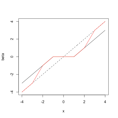
Let’s say we have a response $y \in \mathbb{R}^n$ and a data matrix $X \mathbb{R}^{n \times p}$ , and for simplicity, assume that $y$ and the columns of $X$ are mean-centered. We wish to fit a linear model $y = X \beta$ . In ordinary least squares (OLS), we seek to minimize the objective function

$\underset{\beta}{\min} \quad \| y - X\beta \|_2^2,$

where $\| x \|_2 = \sqrt{x_1^2 + \dots + x_n^2}$ . When $X$ is rank-deficient, the problem is not identifiable. To fix this, we can use ridge regression (Hoerl & Kennard 1970), which always has a unique solution. Ridge regression minimizes the OLS objective function with a sum-of-squares penalty:

$\underset{\beta}{\min} \quad \| y - X\beta \|_2^2 + \lambda \| \beta \|_2^2.$

$\lambda$ is a tuning parameter, with larger values of $\lambda$ leading to more regularized solutions.

While ridge regression has a unique solution, all the entries of $\beta$ are usually non-zero, meaning that all features need to be included in the model. Sometimes, we prefer to have the model be sparse, i.e. have the response as a function of a small subset of features only. LASSO regression (Tibshirani 1996) achieves this by replacing the sum-of-squares penalty with an $L_1$ penalty:

$\underset{\beta}{\min} \quad \| y - X\beta \|_2^2 + \lambda \| \beta \|_1,$

where $\|x\|_1 = |x_1| + \dots + |x_n|$ . The “pointyness” of the $L_1$ ball forces some entries of $\beta$ to be exactly zero when $\lambda$ is large enough.

The LASSO does have its limitations. When $p > n$ , the LASSO can select at most $n$ variables. If there are a group of variables which are highly correlated with each other, the LASSO will tend to just pick one of them. To fix these issues, elastic net regression (Zou & Hastie 2005) have both an $L_1$ penalty and a sum-of-squares penalty:

$\underset{\beta}{\min} \quad \| y - X\beta \|_2^2 + \lambda_1 \| \beta \|_1 + \lambda_2 \| \beta \|_2^2.$

Here, $\lambda_1$ and $\lambda_2$ are both tuning parameters.

Another feature of the LASSO is that it is a shrinkage estimator, i.e. coefficients are shrunk toward zero. This can lead to poorer prediction performance. What we could do instead is use the LASSO as a variable selection tool, then do ordinary least squares on just the selected variables. The relaxed LASSO (Meinshausen 2006) does a more flexible version of that by minimizing

$\underset{\beta}{\min} \quad \dfrac{1}{n} \displaystyle\sum_{i=1}^n ( Y_i - X_i^T \{ \beta \cdot 1_{\mathcal{M}_\lambda} \})^2 + \phi \lambda \| \beta \|_1,$

where $\lambda$ is the parameter controlling variable selection, $\phi \in (0, 1]$ is the parameter controlling the shrinkage of the coefficients, and $1_{\mathcal{M}_\lambda}$ is the indicator function on the set of variables $\mathcal{M}_\lambda \subseteq \{1, \dots, p \}$ so that $\{\beta \cdot 1_{\mathcal{M}_\lambda} \}_k = \beta_k$ if $k \in \mathcal{M}_\lambda$ , $0$ otherwise. When $\phi = 1$ , we obtain the LASSO solution and as $\phi \rightarrow 0$ , we obtain the OLS solution for the selected variables.

It is known that the LASSO is not selection consistent (see Zhao & Yu 2006). A variation of the LASSO that fixes this is the adaptive LASSO (Zou 2006). Let $\hat{\beta}$ be the ordinary least squares solution. (Actually it just needs to be a $\sqrt{n}$ -consistent estimator for the true model coefficients $\beta^*$ .) The adaptive lasso minimizes

$\underset{\beta}{\min} \quad \| y - X\beta \|_2^2 + \lambda \displaystyle\sum_{j =1}^p w_j | \beta_j |,$

where $w_j = 1 / |\hat{\beta}_j|^\gamma$ for some hyperparameter $\gamma > 0$ . The adaptive LASSO is selection consistent (under some assumptions).

In certain cases, we may want a group of variables to all be in the model, or all be out of the model. An example of this is a set of dummy variables. For example, if we have 3 columns representing features $\text{Annual Income } < \$40k$ , $\text{Annual Income } \in [\$40k, \$100k]$ and $\text{Annual Income } > \$100k$ , we may want all 3 to be in the model or all 3 to be out of the model, but not just 1 of them in the model. The group LASSO (Yuan & Lin 2005) achieves this by imposing an $L_2$ penalty on groups of coefficients. Let $G$ be a partition of $\{ 1, \dots, p \}$ , i.e. $\bigcup_{g \in G} g = \{ 1, \dots, p \}$ . The group LASSO minimizes

$\underset{\beta}{\min} \quad \| y - X\beta \|_2^2 + \displaystyle\sum_{g \in G} \lambda_g \| \beta_g \|_2.$

The weights are often chosen as $\lambda_g = \lambda \sqrt{|g|}$ .

While the group LASSO promotes sparsity of groups, once a group is selected for the model, all the coefficients in that group are usually non-zero. To promote both sparsity of groups as well as sparsity within groups, the sparse group LASSO (Simon et al. 2013) imposes a convex combination of the LASSO and group LASSO penalties, minimizing

$\underset{\beta}{\min} \quad \dfrac{1}{2n} \| y - X\beta \|_2^2 + (1 - \alpha)\lambda \displaystyle\sum_{g \in G} \sqrt{|g|} \|\beta_g\|_2 + \alpha \lambda \|\beta\|_1,$

where $\alpha \in [0,1]$ is a parameter.

Statistical Odds & Ends

Tag Archives: regularization

Bayesian Additive Regression Trees (BART)

The minimax concave penalty (MCP)

What is “structured elastic net”?

The SCAD penalty

Different types of regularization