What is a probability-generating function (PGF)?

Posted on November 10, 2025 by kjytay

If $X$ is a discrete random variable taking values in $\{0, 1, \dots \}$ , then the probability-generating function (PGF) of $X$ is defined as

$\begin{aligned} G(z) = \mathbb{E} [z^X] = \sum_{x=0}^\infty p(x) z^x, \end{aligned}$

where $p$ is the probability mass function of $X$ .

PGFs obey all rules of power series with non-negative coefficients. In particular,

$G(1^-) = \lim_{x \uparrow 1} G(x) = 1$ , and
The radius of convergence of a PGF is at least 1.

PGFs can be useful for computing probabilities and expectations:

$\begin{aligned} p(k) = \mathbb{P}\{ X = k\} = \dfrac{G^{(k)}(0)}{k!}. \end{aligned}$

For $k = 0, 1, 2,\dots$ ,

$\begin{aligned} \mathbb{E}\left[ \dfrac{X!}{(X-k)!} \right] = G^{(k)}(1^-) \end{aligned}$

In particular,

$\begin{aligned} \mathbb{E}[X] &= G'(1-), \\ \text{Var}(X) &= G''(1^-) + G'(1^-) - [G'(1^-)]^2. \end{aligned}$

References:

Wikipedia. Probability-generating function.

Brainteaser about points belonging to the same semicircular arc

Posted on August 31, 2025 by kjytay

$n$ points are placed uniformly at random on a circle. What’s the probability that all $n$ of them lie within a semicircular arc?

Label the points $1, 2, \dots, n$ . For each $i =1, \dots, n$ , define the event $A_i$ as the event where all $n$ points lie on the semicircular arc starting from point $i$ and moving clockwise.

The first thing to note is that

$\begin{aligned} \{ \text{all } n \text{ points lie within a semicircular arc} \} = \bigcup_{i=1}^n A_i. \end{aligned}$

The next thing to note is that the $A_i$ ‘s are actually disjoint (except possibly for configurations with probability zero)! We can prove this by contradiction. Assume that $A_i$ and $A_j$ are not disjoint. That means that there is some configuration of points where the clockwise semicircle starting from $i$ covers all points, and the clockwise semicircle starting from $j$ covers all points. Consider moving clockwise from $i$ : the arc reaching $j$ from this direction is $\leq$ half the circle. But by the same logic, the arc reaching $i$ from $j$ in this direction is also $\leq$ half the circle! The only way this is possible is if the two points are two ends of the same diameter, but that happens with probability zero.

Hence,

$\begin{aligned} \mathbb{P}\{ \text{all } n \text{ points lie within a semicircular arc} \} &= \mathbb{P} \left( \bigcup_{i=1}^n A_i \right) \\ &= \sum_{i=1}^n \mathbb{P}(A_i) \\ &= n \mathbb{P} (A_1) \\ &= \frac{n}{2^{n-1}}. \end{aligned}$

Brainteaser about expected number of rolls

Posted on August 30, 2025 by kjytay

An $n$ -sided fair die is rolled repeatedly. What is the expected number of rolls until the total sum becomes at least $n$ ?

This question can be solved by conditioning on the outcome of the first roll. For $k = 1, \dots, n$ , let $E_k$ be the expected number of rolls until the total sum becomes at least $k$ . What we want is $E_n$ .

Let’s evaluate $E_k$ for small $k$ . It’s clear that $E_1 = 1$ , and

$\begin{aligned} E_2 &= \mathbb{P}(\text{roll more than 1}) + \mathbb{P}(\text{roll a 1}) \cdot (1 + E_1) \\ &= \frac{n-1}{n} + \frac{1}{n}(2) \\ &= \frac{n+1}{n}. \end{aligned}$

We can show by induction that $E_k = \left(\dfrac{n+1}{n} \right)^{k-1}$ . Here’s the induction step going from $k-1$ to $k$ :

$\begin{aligned} E_k &= \mathbb{P}(\text{roll more than } k-1) + \sum_{i = 1}^{k-1} \mathbb{P}(\text{roll a } k - i) \cdot (1 + E_i) \\ &= \frac{n-k-1}{n} + \sum_{i=1}^{k-1} \frac{1}{n}\cdot \left[ 1 + \left(\frac{n+1}{n} \right)^{i-1} \right] \\ &= 1 + \frac{1}{n}\sum_{i=1}^{k-1} \left(\frac{n+1}{n} \right)^{i-1} \\ &= 1 + \frac{1}{n} \cdot \frac{(\frac{n+1}{n})^{k-1} - 1}{\frac{n+1}{n} - 1} \\ &= 1+ \left( \frac{n+1}{n} \right)^{k-1} - 1 \\ &= \left( \frac{n+1}{n} \right)^{k-1}. \end{aligned}$

Substituting $k = n$ , we get

$\begin{aligned} E_n = \left( \frac{n+1}{n} \right)^{n-1}. \end{aligned}$

As $n \rightarrow \infty$ , $E_n \rightarrow e$ .

Here’s an R script to check our expression for $E_k$ via Monte Carlo:

run_simulation <- function(n, k) {
  num_rolls <- 0
  current_sum <- 0
  while (current_sum < k) {
    num_rolls <- num_rolls + 1
    current_sum <- current_sum + sample(n, 1)
  }
  
  num_rolls
}

n <- 10
k <- 3
n_sim <- 10000

set.seed(1)
num_rolls <- replicate(n_sim, run_simulation(n, k))
print(paste("MC estimate:", mean(num_rolls)))
print(paste("Exact value:", (1 + 1/n)^(k-1)))

Downloading datasets from Our World in Data in R

Posted on January 30, 2025 by kjytay

I recently learned from Allen Downey’s blog that Our World in Data is providing API access to their data. Our World in Data hosts datasets across several important topics, from population and demographic change, poverty and economic development, to human rights and democracy. From Nov 2024, Our World in Data “[offers] direct URLs to access data in CSV format and comprehensive metadata in JSON format” (this is what they call the Public Chart API).

See this link for full documentation on the chart data API. Allen Downey’s blog post shows how to use this API in Python; in this post I’ll show the corresponding code in R.

Downloading metadata

The chart data API page tells us what APIs are available to us. The starting point is a base URL which we denote by <base_url>. This is what’s available to us:

<base_url> – The page on the website where you can see the chart.
<base_url>.csv – The data for this chart, usually what we want to download.
<base_url>.metadata.json – The metadata for this chart, e.g. chart title, the units, how to cite the data sources.
<base_url>.zip – The dataset, metadata, and a readme as zip file.

Let’s start by looking at the metadata for average monthly surface temperature:

library(tidyverse)
library(httr)
library(jsonlite)

# define URL and query parameters
url <- "https://ourworldindata.org/grapher/average-monthly-surface-temperature.metadata.json"
query_params <- list(
  v = "1",
  csvType = "full",
  useColumnShortNames = "true"
)

# get metadata
headers <- add_headers(`User-Agent` = "Our World In Data data fetch/1.0")
response <- GET(url, query = query_params, headers)
metadata <- fromJSON(content(response, as = "text", encoding = "UTF-8"))

The returned metadata object is a list with a few keys:

# view the metadata keys
names(metadata)

#> [1] "chart"          "columns"        "dateDownloaded" "activeFilters"

The chart element gives us high-level information of the chart:

glimpse(metadata$chart)

#> List of 5
#>  $ title           : chr "Average monthly surface temperature"
#>  $ subtitle        : chr "The temperature of the air measured 2 meters above the ground, encompassing land, sea, and in-land water surfaces."
#>  $ citation        : chr "Contains modified Copernicus Climate Change Service information (2025)"
#>  $ originalChartUrl: chr "https://ourworldindata.org/grapher/average-monthly-surface-temperature?v=1&csvType=full&useColumnShortNames=true"
#>  $ selection       : chr "World"

There’s more information on the dataset in metadata$columns$temperature_2m

names(metadata$columns$temperature_2m)
#>  [1] "titleShort"            "titleLong"             "descriptionShort"      "descriptionProcessing" "shortUnit"             "unit"                 
#>  [7] "timespan"              "type"                  "owidVariableId"        "shortName"             "lastUpdated"           "citationShort"        
#> [13] "citationLong"          "fullMetadata"

(Why temperature_2m? Looking at metadata$columns$temperature_2m$shortName, it seems like temperature_2m is the short name for the dataset.)

Downloading the dataset

Here is code downloading the average monthly surface temperature for just the USA:

# define the URL and query parameters
url <- "https://ourworldindata.org/grapher/average-monthly-surface-temperature.csv"
query_params <- list(
  v = "1",
  csvType = "filtered",
  useColumnShortNames = "true",
  tab = "chart",
  country = "USA"
)

# get data
headers <- add_headers(`User-Agent` = "Our World In Data data fetch/1.0")
response <- GET(url, query = query_params, headers)
df <- read_csv(content(response, as = "text", encoding = "UTF-8"))

head(df)
#> # A tibble: 6 × 6
#>   Entity        Code   year Day        temperature_2m...5 temperature_2m...6
#>   <chr>         <chr> <dbl> <date>                  <dbl>              <dbl>
#> 1 United States USA    1941 1941-12-15            -1.88                 8.02
#> 2 United States USA    1942 1942-01-15            -4.78                 7.85
#> 3 United States USA    1942 1942-02-15            -3.87                 7.85
#> 4 United States USA    1942 1942-03-15             0.0978               7.85
#> 5 United States USA    1942 1942-04-15             7.54                 7.85
#> 6 United States USA    1942 1942-05-15            12.1                  7.85

Allen Downey notes that the last column is undocumented, and based on context is probably the average annual temperature.

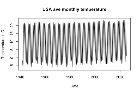
Here’s a simple plot of the data:

plot(df$Day, df$temperature_2m...5, type = "l",
     main = "USA ave monthly temperature",
     xlab = "Date", ylab = "Temperature in C")

If you wanted the entire dataset, just use csvType = "full" in the request parameters, like so:

# define the URL and query parameters
url <- "https://ourworldindata.org/grapher/average-monthly-surface-temperature.csv"
query_params <- list(
  v = "1",
  csvType = "full",
  useColumnShortNames = "true",
  tab = "chart"
)

# same code for the http request works, see above

How do you know which filters you can apply? There is no extensive documentation of what filters you can apply, but as you click on the base URL to change the chart, the URL changes. You can then use this to infer the query parameters to add.

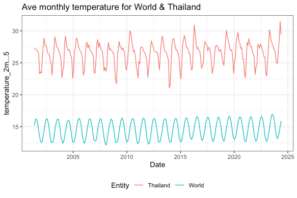
For example, I clicked around on the chart to get this URL: https://ourworldindata.org/grapher/average-monthly-surface-temperature?tab=chart&time=2001-05-15..2024-05-15&country=OWID_WRL~THA. The code below shows how you can download the data and reproduce the chart:

# define the URL and query parameters
url <- "https://ourworldindata.org/grapher/average-monthly-surface-temperature.csv"
query_params <- list(
  v = "1",
  csvType = "filtered",
  useColumnShortNames = "true",
  tab = "chart",
  time = "2001-05-15..2024-05-15",
  country = "OWID_WRL~THA"
)

# get data
headers <- add_headers(`User-Agent` = "Our World In Data data fetch/1.0")
response <- GET(url, query = query_params, headers)
df <- read_csv(content(response, as = "text", encoding = "UTF-8"))
ggplot(df) +
  geom_line(aes(x = Day, y = temperature_2m...5, col = Entity)) +
  labs(title = "Ave monthly temperature for World & Thailand",
       x = "Date", y = "Temperature in C") +
  theme_bw() +
  theme(legend.position = "bottom")

What is the fused lasso?

Posted on January 17, 2025 by kjytay

The fused lasso, introduced in Tibshirani et al. (2005) (Reference 1), is an extension of the lasso. While the lasso produces sparse models, the fused lasso produces models that are not only sparse, but favor a locally constant coefficient profile.

Assume that we have observations $i = 1, \dots, n$ . For each observation $i$ , assume that we have feature data $\boldsymbol{x}_i = ( x_{i1}, x_{i2}, \dots, x_{ip})$ , and an observation $y_i$ which we want to predict. Both the lasso and fused lasso model the predictions as

$\begin{aligned} f(\boldsymbol{x}_i) = \beta_0 + \beta_1 x_{i1} + \dots + \beta_p x_{ip}. \end{aligned}$

Where the methods differ is how they determine the coefficients $\beta_0, \beta_1, \dots, \beta_p$ . The lasso estimates the coefficients as the solution to the minimization problem

$\begin{aligned} \hat\beta = \underset{\beta}{\text{argmin}} \; \left[ \frac{1}{2n} \sum_{i=1}^n \left( y_i - \beta_0 - \sum_{j=1}^p \beta_j x_{ij} \right)^2 + \lambda \sum_{j=1}^p |\beta_j | \right], \end{aligned}$

where $\lambda \geq 0$ is a hyperparameter. (Note that the intercept $\beta_0$ is not included in the penalty term: this is usually the case for regularized models.) The penalty term encourages the coefficients $\beta_j$ to shrink to zero, giving sparsity.

The fused lasso estimates the coefficients as the solution to the minimization problem

$\begin{aligned} \hat\beta = \underset{\beta}{\text{argmin}} \; \left[ \frac{1}{2n} \sum_{i=1}^n \left( y_i - \beta_0 - \sum_{j=1}^p \beta_j x_{ij} \right)^2 + \lambda_1 \sum_{j=1}^p |\beta_j | + \lambda_2 \sum_{j=2}^p |\beta_j - \beta_{j-1} | \right], \end{aligned}$

where $\lambda_1 \geq 0$ and $\lambda_2 \geq 0$ are hyperparameters. On top of penalizing the size of the coefficients, the fused lasso also penalizes the differences between successive coefficients. This encourages the coefficient profile (the plot of $\hat\beta_j$ vs. $j$ ) to look piecewise-constant.

The minimization problem for the fused lasso is a quadratic program and can be solved with general QP solvers. There are of course techniques to make the solver efficient: the original paper (Reference 1) has some ideas. You can fit the fused lasso in R with the fusedlasso function in the genlasso package.

Why might you want to use the fused lasso? You might want to do so when the features are ordered in some meaningful way. Note that the lasso solution is invariant to the ordering of the features whereas the fused lasso solution is not. In Reference 1, they gave a motivating example from protein mass spectroscopy. For a particular sample $i$ , they have intensity values $x_{ij}$ for several mass over charge ratios ( $m/z$ ). The goal is to find $m/z$ -sites that discriminate between healthy and sick patients. The feature number $j$ is related to the $m/z$ value, so it might make sense to have a coefficient profile that is locally constant.

References:

Tibshirani, R., et al. (2005). Sparsity and smoothness via the fused lasso.

What is the Cauchy combination test?

Posted on September 7, 2024 by kjytay

Set-up

Assume that we have p-values $p_1, \dots, p_d$ . Assume that they are computed from z-scores $\mathbf{X} = (X_1, \dots, X_d)$ (test statistics following normal distributions). Let $\mathbb{E}[\mathbf{X}] = \boldsymbol{\mu}$ and let $\text{Cov}(\mathbf{X}) = \mathbf{\Sigma}$ . Without loss of generality, assume that each test statistic $X_i$ has variance 1. With this, we can express the p-values as

$\begin{aligned} p_i = 2 \left[ 1 - \Phi (|X_i|) \right], \end{aligned}$

where $\Phi$ is the CDF function of the standard normal distribution.

We are interested in testing the global null hypothesis $H_0 :\boldsymbol{\mu} = \mathbf{0}$ .

The Cauchy combination test

Assume that we have some random vector $w = (w_1, \dots, w_d)$ such that $w_i \geq 0$ for all $i$ , $w_1 + \dots + w_d = 0$ and $w$ is independent of $\mathbf{X}$ . The test statistic for the Cauchy combination test, proposed by Liu & Xie 2020 (Reference 1), is

$\begin{aligned} T(\mathbf{X}) = \sum_{i=1}^d w_i \tan \left[ \pi \left( 2 \Phi (|X_i|) - \frac{3}{2} \right) \right] = \sum_{i=1}^d w_i \tan \left[ \pi \left( \frac{1}{2} - p_i \right) \right]. \end{aligned}$

Under the global null, $p_i \sim \text{Unif}(0,1)$ for each $i$ , implying that $\tan \left[ \pi \left( \frac{1}{2} - p_i \right) \right]$ has the standard Cauchy distribution (see this previous post). If the p-values are independent, then Proposition 1 in this other previous post implies that $T(\mathbf{X})$ has the standard Cauchy distribution.

In turns out that even if the p-values are dependent, $T(\mathbf{X})$ is still approximately Cauchy! This approximation is formalized in Theorem 1 of Reference 1:

Theorem. Suppose that for any $1 \leq i < j \leq d$ , $(X_i, X_j)$ follows a bivariate normal distribution. Suppose also that $\mathbb{E}[\mathbf{X}] = \mathbf{0}$ . Let $W_0$ be a standard Cauchy random variable. Then for any fixed $d$ and any correlation matrix $\mathbf{\Sigma} \geq \mathbf{0}$ , we have

$\begin{aligned} \lim_{t \rightarrow +\infty} \dfrac{\mathbb{P}\{ T(\mathbf{X}) > t \}}{\mathbb{P} \{ W_0 > t \} } = 1. \end{aligned}$

The theorem says that the test statistic $T(\mathbf{X})$ has approximately a Cauchy tail even under dependency structures in $\mathbf{X}$ . Knowing the (approximate) distribution of $T(\mathbf{X})$ under the global null allows us to use it as a test statistic.

Other notes

The “bivariate normal distribution” condition is a bit of a technical assumption, the authors claim it is a mild assumption.
This result bears a lot of similarity with a result by Pillai & Meng 2016 (see this previous post for a description). Section 2.2 of Reference 1 discusses the similarities and the differences.
Theorem 1 above holds for fixed $d$ (number of p-values). Section 2.3 of Reference 1 has a high-dimensional asymptotic result where $d = o(t^c)$ with $0 < c < 1/2$ .
The Cauchy combination test is especially powerful when only a small number of $\mu_i$ ‘s are large, or equivalently when a smaller number of $p_i$ ‘s are very small. We can see this intuitively: small $p_i$ ‘s become very large $\tan [\pi(1/2 - p_i)]$ ‘s, so the test statistic will be dominated by a few very large p-values. See Section 4.2 of Reference 1 for a power comparison study.

References:

Liu, Y., and Xie, J. (2020). Cauchy Combination Test: A Powerful Test With Analytic p-Value Calculation Under Arbitrary Dependency Structures.

An interesting result involving the Cauchy distribution

Posted on September 7, 2024 by kjytay

If $Z_1, \dots, Z_n$ are independent $\text{Cauchy}(0, 1)$ variables and $w= (w_1, \dots, w_n)$ is a random vector independent of the $Z_i$ ‘s with $w_i \geq 0$ for all $i$ and $w_1 + \dots w_n = 0$ , it is well-known that $\displaystyle\sum_{i=1}^n w_i Z_i$ also has a $\text{Cauchy}(0, 1)$ distribution.

It is also well-known that if $X$ and $Y$ are independent standard normal variables, then $X / Y$ has a $\text{Cauchy}(0, 1)$ distribution.

Putting these two facts together, we have the following proposition:

Proposition 1. Let $\mathbf{X} = (X_1, \dots, X_n)$ and $\mathbf{Y} = (Y_1, \dots, Y_n)$ be i.i.d. $\mathcal{N}(\mathbf{0}, \mathbf{\Sigma})$ , where $\mathbf{\Sigma}$ is a diagonal matrix with strictly positive entries on the diagonal. Let $w = (w_1, \dots, w_n)$ be a random vector independent of $(\mathbf{X},\mathbf{Y})$ such that $w_i \geq 0$ for all $i$ and $w_1 + \dots w_n = 0$ . Then

$\begin{aligned} \sum_{i=1}^n w_i \dfrac{X_j}{Y_j} \sim \text{Cauchy}(0,1). \end{aligned}$

Interestingly, the result above holds for any covariance matrix $\mathbf{\Sigma}$ with positive entries on the diagonal! This was proved in Pillai & Meng 2016 (Reference 1). In other words, we can have any dependence structure between the elements of $\mathbf{X}$ (and likewise for $\mathbf{Y}$ , but as long as the dependence structure for the two random vectors is the same, the linear combination of their ratios remains Cauchy-distributed! Here is the formal statement:

Proposition 2. Let $\mathbf{X} = (X_1, \dots, X_n)$ and $\mathbf{Y} = (Y_1, \dots, Y_n)$ be i.i.d. $\mathcal{N}(\mathbf{0}, \mathbf{\Sigma})$ , where $\mathbf{\Sigma}$ is any covariance matrix with strictly positive entries on the diagonal. Let $w = (w_1, \dots, w_n)$ be a random vector independent of $(\mathbf{X},\mathbf{Y})$ such that $w_i \geq 0$ for all $i$ and $w_1 + \dots w_n = 0$ . Then

$\begin{aligned} \sum_{i=1}^n w_i \dfrac{X_j}{Y_j} \sim \text{Cauchy}(0,1). \end{aligned}$

References:

Pillai, N. S., and Meng, X.-L. (2016). An Unexpected Encounter with Cauchy and Lévy.

Converting a uniform distribution into a Cauchy distribution

Posted on August 29, 2024 by kjytay

The following proposition demonstrates how one can transform a uniform distribution on $(0, 1)$ into a standard Cauchy distribution:

Proposition. If $U \sim \text{Unif}(0,1)$ and $X = \tan \left[ \pi \left( \frac{1}{2} - U \right)\right]$ , then $X$ has standard Cauchy distribution.

Proof: For any $x \in \mathbb{R}$ ,

$\begin{aligned} \mathbb{P} \left\{ X \leq x \right\} &= \mathbb{P} \left\{ \tan \left[ \pi \left( \frac{1}{2} - U \right)\right] \leq x \right\} \\ &= \mathbb{P} \left\{ \frac{1}{2} - U \leq \frac{1}{\pi}\tan^{-1} x \right\} \\ &= \mathbb{P} \left\{ \frac{1}{2} - \frac{1}{\pi}\tan^{-1} x \leq U \right\} \\ &= 1 - \left[ \frac{1}{2} - \frac{1}{\pi}\tan^{-1} x \right] \\ &= \frac{1}{2} + \frac{1}{\pi}\tan^{-1} x, \end{aligned}$

where the second-last equality is due to the fact that $\tan^{-1} x \in (-\frac{1}{2}, \frac{1}{2})$ , so the LHS inside the probability is always in $(0, 1)$ . In other words, $X$ has the CDF of the standard Cauchy distribution.

We could also differentiate the CDF above w.r.t. $x$ to get the PDF of $X$ , which is more easily recognizable as the PDF of the standard Cauchy:

$\begin{aligned} f_X(x) &= \dfrac{d}{dx} \left[ \frac{1}{2} + \frac{1}{\pi}\tan^{-1} x \right] \\ &= \frac{1}{\pi (1 + x^2)}. \end{aligned}$

(Alternatively, one could use the formulas in this previous post with minor modifications since the transformation here is monotonically decreasing, not increasing.)

What is Adam and AdamW?

Posted on June 27, 2024 by kjytay

Adam (short for adaptive moment estimation) was proposed by Kingma & Ba (2014) (Reference 1) as a first-order gradient-based optimization method that combines the advantages of AdaGrad (Duchi et al. 2011, Reference 2) (ability to deal with sparse gradients) and RMSProp (Tieleman & Hinton 2012, Reference 3) (ability to deal with non-stationary objectives). While considered an old method by now, it’s still widely used as a baseline algorithm to compare more cutting-edge algorithms against.

According to the authors,

“Some of Adam’s advantages are that the magnitudes of parameter updates are invariant to rescaling of the gradient, its stepsizes are approximately bounded by the stepsize hyperparameter, it does not require a stationary objective, it works with sparse gradients, and it naturally performs a form of step size annealing.”

Notation

$f : \mathbb{R}^d \mapsto \mathbb{R}$ is a noise objective function that is differentiable w.r.t. to its parameter $\theta$ . We want to minimize $\mathbb{E}[f(\theta)]$ .
$f_1(\theta), \dots, f_T(\theta)$ are stochastic realizations of $f$ at timesteps $1, \dots, T$ .
Let $g_t = \nabla_\theta f_t (\theta)$ denote the gradient of $f_t$ w.r.t. $\theta$ .

Adam

At each timestep $t$ , Adam keeps track of $\hat{m}_t$ , an estimate of the first moment of the gradient $g_t$ , and $\hat{v}_t$ , an estimate of the second raw moment (uncentered variance) of the gradient $g_t^2 = g_t \odot g_t$ ( $\odot$ represents element-wise multiplication). The Adam update is

$\theta_t \leftarrow \theta_{t-1} - \alpha \cdot \hat{m}_t / (\sqrt{\hat{v}_t + \epsilon}),$

where $\alpha$ and $\epsilon$ are hyperparameters. The full description of Adam is in the Algorithm below:

Adam algorithm (Algorithm 1 of Kingma & Ba).

Comparison with other methods

In comparison with Adam, the vanilla SGD update is

$\theta_t \leftarrow \theta_{t-1} - \alpha \cdot g_t ,$

and the classical momentum-based SGD update is

$\theta_t \leftarrow \theta_{t-1} - \alpha \cdot \hat{m}_t.$

The basic version of AdaGrad has update rule

$\begin{aligned} \theta_t \leftarrow \theta_{t-1} - \alpha \cdot g_t / \sqrt{\sum_{i=1}^t g_t^2}. \end{aligned}$

AdaGrad corresponds to Adam with $\beta_1 = 0$ , infinitesimal $(1-\beta_2)$ , and replacing $\alpha$ with $\alpha_t = \alpha \cdot t^{-1/2}$ (see Section 5 of Reference 1 for a few more details).

AdamW

AdamW, proposed by Loshchilov & Hutter 2019 (Reference 4), is a simple modification of Adam which “improves regularization in Adam by decoupling the weight decay from the gradient-based update”.

The original weight decay update was of the form

$\begin{aligned} \theta_{t+1} = (1-\lambda) \theta_t - \alpha g_t, \end{aligned}$

where $\lambda$ defines the rate of weight decay per step. Loshchilov & Hutter (2019) note that for standard SGD, this weight decay is equivalent to L2 regularization (Proposition 1 of Reference 4), but the two are not equivalent for the Adam update. They present Adam with L2 regularization and Adam with decoupled weight decay (AdamW) together in Algorithm 2 of the paper:

Overall, the authors found that AdamW performed better than Adam with L2 regularization.

PyTorch’s implementation of AdamW can be found here.

References:

Kingma, D. P., and Ba, J. (2014). Adam: A Method for Stochastic Optimization.
Duchi, J., et al. (2011). Adaptive Subgradient Methods for Online Learning and Stochastic Optimization.
Tieleman, T., and Hinton, G. (2012). Lecture 6.5 – RMSProp, Coursera: Neural Networks for Machine Learning. (If someone has a link/PDF for the slides, I’d be grateful!)
Loshchilov, I., and Hutter, F. (2019). Decoupled Weight Decay Normalization.

What is elastic weight consolidation?

Posted on June 26, 2024 by kjytay

Elastic weight consolidation (EWC) is a technique proposed by Kirkpatrick et al. (2016) (Reference 1) as a way for avoiding catastrophic forgetting in neural networks.

Set-up and notation

Imagine that we want to train a neural network to be able to perform well on several different tasks. In real-world settings, it’s not always possible to have all the data from all tasks available at the beginning of model training, so we want our model to be able to learn continually: “that is, [have] the ability to learn consecutive tasks without forgetting how to perform previously trained tasks.”

This turns out to be difficult for neural networks because of a phenomenon known as catastrophic forgetting. Assume that I have already trained a model to be good at one task, task A. Now, when I further train this model to be good at a second task, task B, performance on task A tends to degrade, with the performance drop often happening abruptly (hence “catastrophic”). This happens because “the weights in the network that are important for task A are changed to meet the objectives of task B”.

Let’s rewrite the previous paragraph with some mathematical notation. Assume that we have training data $\mathcal{D}_A$ and $\mathcal{D}_B$ for tasks A and B respectively. Let $\mathcal{D} = \mathcal{D}_A \cup \mathcal{D}_B$ . Our neural network is parameterized by $\theta$ : model training corresponds to finding an “optimal” value of $\theta$ .

Let’s say that training on task A gives us the network parameters $\theta_A^\star$ . Catastrophic forgetting says that when further training on task B (to reach new optimal parameters $\theta_B^\star$ ), $\theta_B^\star$ is too far away from $\theta_A^\star$ and hence has poor performance on task A.

Elastic weight consolidation (EWC)

The intuition behind elastic weight consolidation (EWC) is the following: since large neural networks tend to be over-parameterized, it is likely that for any one task, there are many values of $\theta$ that will give similar performance. Hence, when further training on task B, we should constrain the model parameters to be “close” to $\theta_A^\star$ in some sense. The figure below (Figure 1 from Reference 1) illustrates this intuition:How do we make this intuition concrete? Assume that we are in a Bayesian setting. What we would like to do is maximize the (log) posterior probability of $\theta$ given all the data $\mathcal{D}$ :

$\begin{aligned} \log p(\theta | \mathcal{D}) = \log p(\mathcal{D} | \theta) + \log p(\theta) - \log p(\mathcal{D}). \end{aligned}$

Note that the equation above applies if we replace all instances of $\mathcal{D}$ with $\mathcal{D}_A$ or $\mathcal{D}_B$ . Assuming the data for tasks A and B are independent, let’s do some rewriting of the equation above:

$\begin{aligned} \log p(\theta | \mathcal{D}) &= \log p(\mathcal{D}_A | \theta) + \log p(\mathcal{D}_B | \theta) + \log p(\theta) - \log p(\mathcal{D}_A) - \log p(\mathcal{D}_B) \\ &= \log p(\mathcal{D}_B | \theta) + \log p(\theta) - \log p(\mathcal{D}_A) - \log p(\mathcal{D}_B) \\ &\qquad + [\log p(\theta | \mathcal{D}_A) - \log p(\theta) + \log p (\mathcal{D}_A) ] \\ &= \log p(\mathcal{D}_B | \theta) + \log p(\theta | \mathcal{D}_A) - \log p(\mathcal{D}_B). \end{aligned}$

Thus, maximizing the log posterior probability of $\theta$ is equivalent to maximizing

$\log p(\mathcal{D}_B | \theta) + \log p(\theta | \mathcal{D}_A). \qquad -(1)$

Assume that we have already trained our model in some way to get to $\theta_A^\star$ which does well on task A. We recognize the first term above as the log-likelihood function for task B’s training data: maximizing just the first term alone corresponds to the usual maximum likelihood estimation (MLE). For the second term, we can approximate the posterior distribution of $\theta$ based on task A’s data as a Gaussian distribution centered around $\theta_A^\star$ with some covariance. (This is known as the Laplace approximation). Simplifying even further: instead of the distribution having precision matrix equal to the full Fisher information matrix $F$ , we assume that the precision matrix is diagonal having the same values as the diagonal of $F$ .

Putting it altogether, maximizing $(1)$ is equivalent to minimizing

$\mathcal{L}(\theta) = \mathcal{L}_B (\theta) + \sum_i \frac{\lambda}{2} F_i (\theta_i - \theta_{A,i}^\star)^2,$

where $\mathcal{L}_B(\theta)$ is the loss for task B only, $i$ indexes the weights and $\lambda \geq 0$ is an overall hyperparameter that balances the importance of the two tasks. EWC minimizes $\mathcal{L}(\theta)$ .

Why the name “elastic weight consolidation”? From the authors:

“This constraint is implemented as a quadratic penalty, and can therefore be imagined as a spring anchoring the parameters to the previous solution, hence the name elastic. Importantly, the stiffness of this spring should not be the same for all parameters; rather, it should be greater for those parameters that matter most to the performance during task A.”

References:

Kirkpartick, J., et al. (2016). Overcoming catastrophic forgetting in neural networks.