
Introduction
Every year on February 7th, math enthusiasts worldwide (should) consider celebrating Euler’s Day or E-day. Among Euler’s many gifts to the (currently known) mathematical universe is the ever-popular number e, the natural logarithm base that is basically the rock star of calculus, complex analysis, continuous growth models, compound interest, and (much) more. That irrational number shows up in places we might or might not expect. This blog post (notebook) explores some formulas and plots related to Euler’s number, e.
Remark: The code of the fractal plots is Raku translation of the Wolfram Language code in the notebook “Celebrating Euler’s day: algorithms for derangements, branch cuts, and exponential fractals” by Ed Pegg.
Setup
use JavaScript::D3;use JavaScript::D3::Utilities;
#% javascriptrequire.config({ paths: { d3: 'https://d3js.org/d3.v7.min'}}); require(['d3'], function(d3) { console.log(d3);});
#% jsjs-d3-list-line-plot(10.rand xx 40, background => 'none', stroke-width => 2)
my $title-color = 'Silver';my $background = '#1F1F1F';
Formulas and computation
Raku has the built in mathematical constant (base of the natural logarithm). Both ASCII “e” and Unicode “𝑒” (“MATHEMATICAL ITALIC SMALL E” or U+1D452) can be used:
[e, 𝑒]
# [2.718281828459045 2.718281828459045]
We can verify this famous equation:
e ** (i * π) + 1
# 0+1.2246467991473532e-16i
Let us compute using the canonical formula:

Here is the corresponding Raku code:
my @e-terms = ([\*] 1.FatRat .. *);my $e-by-sum = 1 + (1 «/» @e-terms[0 .. 100]).sum
# 2.7182818284590452353602874713526624977572470936999595749669676277240766303535475945713821785251664274274663919320030599218174135966290435729003342952605956307381312
Here we compute the e using Wolfram Language (via wolframscript):
my $proc = run 'wolframscript', '--code', 'N[E, 100]', :out;my $e-wl = $proc.out.slurp(:close).substr(0,*-6).FatRat
# 2.7182818284590452353602874713526624977572470936999595749669676277240766303535475945713821785251664274274661651602106
Side-by-side comparison:
#% html[ {lang => 'Raku', value => $e-by-sum.Str.substr(0,100)}, {lang => 'Wolfram Language', value => $e-wl.Str.substr(0,100)}]==> to-html(field-names => <lang value>, align => 'left')
| lang | value |
|---|---|
| Raku | 2.71828182845904523536028747135266249775724709369995957496696762772407663035354759457138217852516642 |
| Wolfram Language | 2.71828182845904523536028747135266249775724709369995957496696762772407663035354759457138217852516642 |
And here is the absolute difference:
abs($e-by-sum - $e-wl).Num
# 2.2677179245992183e-106
Let us next compute e using the continued fraction formula:

To make the corresponding continued fraction we first generate its sequence using Philippe Deléham formula for OEIS sequence A003417:
my @rec = 2, 1, 2, 1, 1, 4, 1, 1, -1 * * + 0 * * + 0 * * + 2 * * + 0 * * + 0 * * ... Inf;@rec[^20]
# (2 1 2 1 1 4 1 1 6 1 1 8 1 1 10 1 1 12 1 1)
Here is a function that computes the continuous fraction formula:
sub e-by-cf(UInt:D $i) { @rec[^$i].reverse».FatRat.reduce({$^b + 1 / $^a}) }
Remark: A more generic continued fraction computation is given in the Raku entry for “Continued fraction”.
Let us compare all three results:
#% html[ {lang => 'Raku', formula => 'sum', value => $e-by-sum.Str.substr(0,100)}, {lang => 'Raku', formula => 'cont. fraction', value => &e-by-cf(150).Str.substr(0,100)}, {lang => 'WL', formula => '-', value => $e-wl.Str.substr(0,100)}]==> to-html(field-names => <lang formula value>, align => 'left')
| lang | formula | value |
|---|---|---|
| Raku | sum | 2.71828182845904523536028747135266249775724709369995957496696762772407663035354759457138217852516642 |
| Raku | cont. fraction | 2.71828182845904523536028747135266249775724709369995957496696762772407663035354759457138217852516642 |
| WL | – | 2.71828182845904523536028747135266249775724709369995957496696762772407663035354759457138217852516642 |
Plots
The maximum of the function x^(1/x) is attained at e:
#% jsjs-d3-list-line-plot((1, 1.01 ... 5).map({ [$_, $_ ** (1/$_)] }), :$background, stroke-width => 4, :grid-lines)

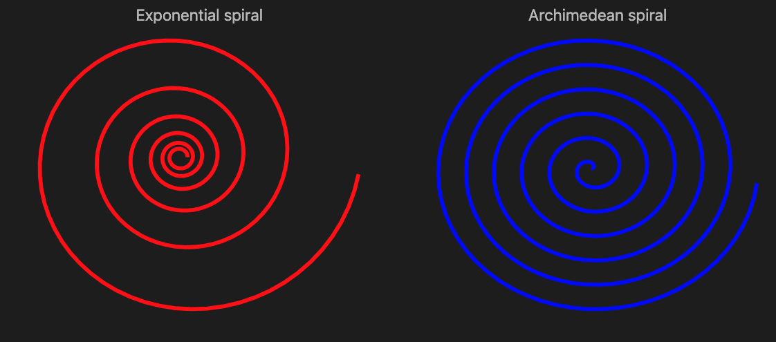
The Exponential spiral is based on the exponential function (and below it is compared to the Archimedean spiral):
#% jsmy @log-spiral = (0, 0.1 ... 12 * π).map({ e ** ($_/12) «*» [cos($_), sin($_)] });my @arch-spiral = (0, 0.1 ... 12 * π).map({ 2 * $_ «*» [cos($_), sin($_)] });my %opts = stroke-width => 4, :!axes, :!grid-lines, :400width, :350height, :$title-color;js-d3-list-line-plot(@log-spiral, :$background, color => 'red', title => 'Exponential spiral', |%opts) ~js-d3-list-line-plot(@arch-spiral, :$background, color => 'blue', title => 'Archimedean spiral', |%opts)
Catenary is the curve a hanging flexible wire or chain assumes when supported at its ends and acted upon by a uniform gravitational force. It is given with the formula:
Here is a corresponding plot:
#% jsjs-d3-list-line-plot((-1, -0.99 ... 1).map({ [$_, e ** $_ + e ** (-$_)] }), :$background, stroke-width => 4, :grid-lines, title => 'Catenary curve', :$title-color)

Fractals
The exponential curlicue fractal:
#%jsjs-d3-list-line-plot(angle-path(e <<*>> (1...15_000)), :$background, :!axes, :400width, :600height)

Here is a plot of exponential Mandelbrot set:
my $h = 0.01;my @table = do for -2.5, -2.5 + $h ... 2.5 -> $x { do for -1, -1 + $h ... 4 -> $y { my $z = 0; my $count = 0; while $count < 30 && $z.abs < 10e12 { $z = exp($z) + $y + $x * i; $count++; } $count - 1; }}deduce-type(@table)
#% jsjs-d3-matrix-plot(@table, :!grid-lines, color-palette => 'Rainbow', :!tooltip, :!mesh)

A fractal variant using reciprocal:
my $h = 0.0025;my @table = do for -1/2, -1/2 + $h ... 1/6 -> $x { do for -1/2, -1/2 + $h ... 1/2 -> $y { my $z = $x + $y * i; my $count = 0; while $count < 10 && $z.abs < 100000 { $z = exp(1 / $z); $count++; } $count; }}deduce-type(@table)
#% jsjs-d3-matrix-plot(@table, :!grid-lines, color-palette => 'Rainbow', :!tooltip, :!mesh)

