Pi Day 2026: Formulas, Series, and Plots for π

Introduction

  • Happy Pi Day! Today (3/14) we celebrate the most famous mathematical constant: π ≈ 3.141592653589793…
  • π is irrational and transcendental, appears in circles, waves, probability, physics, and even random walks.
  • Raku (with its built-in π constant, excellent rational support, lazy lists, and unicode operators) makes experimenting with π relatively easy and enjoyable.
  • In this blog post (notebook) we explore a selection of formulas and algorithms.

0. Setup

use Math::NumberTheory;
use BigRoot;
use Image::Markup::Utilities;
use Graphviz::DOT::Chessboard;
use Data::Reshapers;
use JavaScript::D3;
use JavaScript::D3::Utilities;

D3.js

#%javascript
require.config({
paths: {
d3: 'https://d3js.org/d3.v7.min'
}});
require(['d3'], function(d3) {
console.log(d3);
});
my $title-color = 'Ivory';
my $stroke-color = 'SlateGray';

1. Continued fraction approximation

The built-in Raku constant pi (or π) is fairly low precision:

say π.fmt('%.25f')
# 3.1415926535897930000000000

One way to remedy that is to use continued fractions. For example, using the (first) sequence line of On-line Encyclopedia of Integer Sequences (OEIS) A001203 produces  with precision 56:

my @s = 3, 7, 15, 1, 292, 1, 1, 1, 2, 1, 3, 1, 14, 2, 1, 1, 2, 2, 2, 2, 1, 84, 2, 1, 1, 15, 3, 13, 1, 4, 2, 6, 6, 99, 1, 2, 2, 6, 3, 5, 1, 1, 6, 8, 1, 7, 1, 2, 3, 7, 1, 2, 1, 1, 12, 1, 1, 1, 3, 1, 1, 8, 1, 1, 2, 1, 6, 1, 1, 5, 2, 2, 3, 1, 2, 4, 4, 16, 1, 161, 45, 1, 22, 1, 2, 2, 1, 4, 1, 2, 24, 1, 2, 1, 3, 1, 2, 1;
my $pi56 = from-continued-fraction(@s».FatRat.List);
# 3.14159265358979323846264338327950288419716939937510582097

Here we verify the precision using Wolfram Language:

"wolframscript -code 'N[Pi, 100] - $pi56'"
andthen .&shell(:out)
andthen .out.slurp(:close)
# 0``56.

More details can be found in Wolfram MathWorld page “Pi Continued Fraction”, [EW1].


2. Continued fraction terms plots

It is interesting to consider the plotting the terms of continued fraction terms of .

First we ingest the more “pi-terms” from OEIS A001203 (20k terms):

my @ds = data-import('https://oeis.org/A001203/b001203.txt').split(/\s/)».Int.rotor(2);
my @terms = @ds».tail;
@terms.elems
# 20000

Here is the summary:

sink records-summary(@terms)
# +-------------------+
# | numerical |
# +-------------------+
# | 1st-Qu => 1 |
# | Median => 2 |
# | Min => 1 |
# | Max => 20776 |
# | Mean => 12.6809 |
# | 3rd-Qu => 5 |
# +-------------------+

Here is an array plot of the first 128 terms of the continued fraction approximating :

#% html
my @mat = |@terms.head(128)».&integer-digits(:2base);
my $max-digits = @mat».elems.max;
@mat .= map({ [|(0 xx (``max-digits - ``_.elems)), |$_] });
dot-matrix-plot(transpose(@mat), size => 10):svg
cell 26 output 1 svg 1

Next, we show the Pareto principle manifestation of for the continued fraction terms. First we observe that the terms a distribution similar to Benford’s law:

#% js
my @tally-pi = tally(@terms).sort(-*.value).head(16) <</>> @terms.elems;
my @terms-b = random-variate(BenfordDistribution.new(:10base), 2_000);
my @tally-b = tally(@terms-b).sort(-*.value).head(16) <</>> @terms-b.elems;
js-d3-bar-chart(
[
|@tally-pi.map({ %( x => ``_.key, y => ``_.value, group => 'π') }),
|@tally-b.map({ %( x => ``_.key, y => ``_.value, group => 'Benford') })
],
plot-label => "Pi continued fraction terms vs. Benford's law",
:$title-color,
:$background)

Here is the Pareto principle plot — ≈5% of the unique term values correspond to ≈80% of the terms:

#% js
js-d3-list-line-plot(
pareto-principle-statistic(@terms),
plot-label => "Pi continued fraction terms vs. Benford's law",
:$title-color,
:$background,
stroke-width => 5,
:grid-lines
)

3. Classic Infinite Series

Many ways to express π as an infinite sum — some converge slowly, others surprisingly fast.

Leibniz–Gregory series (1671/ Madhava earlier)

Raku implementation:

sub pi-leibniz($n) {
4 * [+] map { (``_ %% 2 ?? 1 !! -1) / (2 * ``_.FatRat + 1) }, 0 ..^ $n
}
my $piLeibniz = pi-leibniz(1_000);
# 3.140592653839792925963596502869395970451389330779724489367457783541907931239747608265172332007670207231403885276038710899938066629552214564551237742887150050440512339302537072825852760246628025562008569471700451065826106184744099667808080815231833582150382088582680381403109153574884416966097481526954707518119416184546424446286573712097944309435229550466609113881892172898692240992052089578302460852737674933105951137782047028552762288434104643076549100475536363928011329215789260496788581009721784276311248084584199773204673225752150684898958557383759585526225507807731149851003571219339536433193219280858501643712664329591936448794359666472018649604860641722241707730107406546936464362178479780167090703126423645364670050100083168338273868059379722964105943903324595829044270168232219388683725629678859726914882606728649659763620568632099776069203461323565260334137877

Verify with Wolfram Language (again):

"wolframscript -code 'N[Pi, 1000] - $piLeibniz'"
andthen .&shell(:out)
andthen .out.slurp(:close)
# 0.000999999750000312499...814206`866.9999998914263

Nilakantha series (faster convergence):

Raku:

sub pi-nilakantha($n) {
3 + [+] map {
($_ %% 2 ?? -1 !! 1 ) * 4 / ((2 * $_.FatRat) * (2 * $_ + 1) * (2 * $_ + 2))
}, 1 .. $n
}
pi-nilakantha(1_000);
# 3.141592653340542051900128736253203567152539255317954874674304859504426172618558702218695071137605738966036069683335561974900086119307836254205910905806190030949758215864755464129701335459521079534522811851010296642538249613529207613335816447914992502190861349451746347920350033634355181084537761886275546599078437173552420948534950023442771396391252038722980428723971632669306434394851189528826699233048019261441283970866004550291393472342649870962106821115715774722114776992400455398838055772839725805047379519366309217982783671029012753365224924699602163737619311405432798527164991008945233085366633073462699045511265528492985424805854418596455931463431855615794431867539190155631617285217459790661344075940516099637034367441911754544671168909454186231972510120715400925996293656987342326715209388299050131213232932065481743222390684073879385764855135985734675127240826
"wolframscript -code 'N[Pi, 1000] - {pi-nilakantha(1_000)}'"
andthen .&shell(:out)
andthen .out.slurp(:close)
# 2.4925118...83814206`860.3966372344514*^-10

3. Beautiful Products

Wallis product (1655) — elegant infinite product:

Raku running product:

my $p = 2.0;
for 1 .. 1_000 -> $n {
``p *= (2 * ``n) * (2 * ``n) / ( (2 * ``n - 1 ) * ( 2 * $n + 1) );
say "``n → {``p / ``piLeibniz} relative error" if ``n %% 100;
}
# 100 → 0.9978331595460779 relative error
# 200 → 0.9990719099195204 relative error
# 300 → 0.9994865459690567 relative error
# 400 → 0.9996941876848563 relative error
# 500 → 0.9998188764663584 relative error
# 600 → 0.9999020455903246 relative error
# 700 → 0.9999614733132168 relative error
# 800 → 1.0000060557070767 relative error
# 900 → 1.0000407377794782 relative error
# 1000 → 1.000068487771041 relative error

4. Very Fast Modern Series — Chudnovsky Algorithm

One of the fastest-converging series used in record computations:

Each term adds roughly 14 correct digits. Cannot be implemented easily in Raku, since Raku does not have bignum sqrt and power operations.


5. Spigot Algorithms — Digits “Drip” One by One

Spigot algorithms compute decimal digits using only integer arithmetic — no floating-point errors accumulate.

The classic Rabinowitz–Wagon spigot (based on a transformed Wallis product) produces base-10 digits sequentially.

Simple (but bounded) version outline in Raku:

sub spigot-pi($digits) {
my ``len = (10 * ``digits / 3).floor + 1;
my @a = 2 xx $len;
my @result;
for 1..$digits {
my $carry = 0;
for ``len-1 ... 0 -> ``i {
my ``x = 10 * @a[``i] + ``carry * (``i + 1);
@a[``i] = ``x % (2 * $i + 1);
``carry = ``x div (2 * $i + 1);
}
@result.push($carry div 10);
@a[0] = $carry % 10;
# (handle carry-over / nines adjustment in full impl)
}
@result.head(1).join('.') ~ @result[1..*].join
}
spigot-pi(50);
# 314159265358979323846264338327941028841971693993751
"wolframscript -code 'N[Pi, 100] - {spigot-pi(50).FatRat / 10e49.FatRat}'"
andthen .&shell(:out)
andthen .out.slurp(:close)
# 2.3969628881355243801510070603398913366797194459230781640628621`41.37966130996076*^-16

6. BBP Formula — Hex Digits Without Predecessors

Bailey–Borwein–Plouffe (1995) formula lets you compute the nth hexadecimal digit of π directly (without earlier digits):

Very popular for distributed π-hunting projects. The best known digit-extraction algorithm.

Raku snippet for partial sum (base 16 sense):

sub bbp-digit-sum($n) {
[+] (0..$n).map: -> $k {
my $r = 1/16**$k;
$r * (4/(8*$k+1) - 2/(8*$k+4) - 1/(8*$k+5) - 1/(8*$k+6))
}
}
say bbp-digit-sum(100).base(16).substr(0,20);
# 3.243F6B

7. (Instead of) Conclusion

  • π contains (almost surely) every finite sequence of digits — your birthday appears infinitely often.
  • The Feynman point: six consecutive 9s starting at digit 762.
  • Memorization world record > 100,000 digits.
  • π appears in the normal distribution, quantum mechanics, random walks, Buffon’s needle problem (probability ≈ 2/π).

Let us plot a random walk using the terms of continued fraction of Pi — the 20k or OEIS A001203 — to determine directions:

#% js
my @path = angle-path(@terms)».reverse».List;
my &pi-path-map = {
given @terms[$_] // 0 {
when $_ ≤ 100 { 0 }
when $_ ≤ 1_000 { 1 }
default { 2 }
}
}
@path = @path.kv.map( -> $i, $p {[|$p, &pi-path-map($i).Str]});
my %opts = color-scheme => 'Observable10', background => '#1F1F1F', :!axes, :!legends, stroke-width => 2;
js-d3-list-line-plot(@path, :800width, :500height, |%opts)

In the plot above the blue segments correspond to origin terms ≤ 100, yellow segments to terms between 100 and 1000, and red segment for origin terms greater than 1000.


References

[EW1] Eric Weisstein, “Pi Continued Fraction”Wolfram MathWorld.

Jupyter::Chatbook Cheatsheet

Quick reference for the Raku package “Jupyter::Chatbook”. (raku.landGitHub.)


0) Preliminary steps

Follow the instructions in the README of “Jupyter::Chatbook”:

For installation and setup problems see the issues (both open and closed) of package’s GitHub repository.
(For example, this comment.)


1) New LLM persona initialization

A) Create persona with #%chat or %%chat (and immediately send first message)

#%chat assistant1, name=ChatGPT model=gpt-4.1-mini prompt="You are a concise technical assistant."
Say hi and ask what I am working on.
# Hi! What are you working on?

Remark: For all “Jupyter::Chatbook” magic specs both prefixes %% and #% can be used.

Remark: For the prompt argument the following delimiter pairs can be used: '...'"..."«...»{...}⎡...⎦.

B) Create persona with #%chat <id> prompt (create only)

#%chat assistant2 prompt, conf=ChatGPT, model=gpt-4.1-mini
You are a code reviewer focused on correctness and edge cases.
# Chat object created with ID : assistant2.

You can use prompt specs from “LLM::Prompts”, for example:

#%chat yoda prompt
@Yoda
# Chat object created with ID : yoda.
Expanded prompt:
⎡You are Yoda.
Respond to ALL inputs in the voice of Yoda from Star Wars.
Be sure to ALWAYS use his distinctive style and syntax. Vary sentence length.⎦

The Raku package “LLM::Prompts” (GitHub link) provides a collection of prompts and an implementation of a prompt-expansion Domain Specific Language (DSL).


2) Notebook-wide chat with an LLM persona

Continue an existing chat object

Render the answer as Markdown:

#%chat assistant1 > markdown
Give me a 5-step implementation plan for adding authentication to a FastAPI app. VERY CONCISE.

Magic cell parameter values can be assigned using the equal sign (“=”):

#%chat assistant1 > markdown
Now rewrite step 2 with test-first details.

Default chat object (NONE)

#%chat
Does vegetarian sushi exist?
# Yes, vegetarian sushi definitely exists! It's a popular option for those who avoid fish or meat. Instead of raw fish, vegetarian sushi typically includes ingredients like:
- Avocado
- Cucumber
- Carrots
- Pickled radish (takuan)
- Asparagus
- Sweet potato
- Mushrooms (like shiitake)
- Tofu or tamago (Japanese omelette)
- Seaweed salad
These ingredients are rolled in sushi rice and nori seaweed, just like traditional sushi. Vegetarian sushi can be found at many sushi restaurants and sushi bars, and it's also easy to make at home.

Using the prompt-expansion DSL to modify the previous chat-cell result:

#%chat
!HaikuStyled>^
# Rice, seaweed embrace,
Avocado, crisp and bright,
Vegetarian.

3) Management of personas (#%chat <id> meta)

Query one persona

#%chat assistant1 meta
prompt
# "You are a concise technical assistant."
#%chat assistant1 meta
say
# Chat: assistant1
# ⸺⸺⸺⸺⸺⸺⸺⸺⸺⸺⸺⸺⸺⸺⸺⸺⸺⸺⸺⸺⸺⸺⸺⸺⸺⸺⸺⸺⸺⸺⸺⸺⸺⸺⸺⸺⸺⸺⸺⸺⸺⸺⸺⸺⸺⸺⸺⸺⸺⸺⸺⸺⸺⸺⸺⸺⸺⸺⸺⸺
# Prompts: You are a concise technical assistant.
# ⸺⸺⸺⸺⸺⸺⸺⸺⸺⸺⸺⸺⸺⸺⸺⸺⸺⸺⸺⸺⸺⸺⸺⸺⸺⸺⸺⸺⸺⸺⸺⸺⸺⸺⸺⸺⸺⸺⸺⸺⸺⸺⸺⸺⸺⸺⸺⸺⸺⸺⸺⸺⸺⸺⸺⸺⸺⸺⸺⸺
# role : user
# content : Say hi and ask what I am working on.
# timestamp : 2026-03-14T09:23:01.989418-04:00
# ⸺⸺⸺⸺⸺⸺⸺⸺⸺⸺⸺⸺⸺⸺⸺⸺⸺⸺⸺⸺⸺⸺⸺⸺⸺⸺⸺⸺⸺⸺⸺⸺⸺⸺⸺⸺⸺⸺⸺⸺⸺⸺⸺⸺⸺⸺⸺⸺⸺⸺⸺⸺⸺⸺⸺⸺⸺⸺⸺⸺
# role : assistant
# content : Hi! What are you working on?
# timestamp : 2026-03-14T09:23:03.222902-04:00
# ⸺⸺⸺⸺⸺⸺⸺⸺⸺⸺⸺⸺⸺⸺⸺⸺⸺⸺⸺⸺⸺⸺⸺⸺⸺⸺⸺⸺⸺⸺⸺⸺⸺⸺⸺⸺⸺⸺⸺⸺⸺⸺⸺⸺⸺⸺⸺⸺⸺⸺⸺⸺⸺⸺⸺⸺⸺⸺⸺⸺
# role : user
# content : Give me a 5-step implementation plan for adding authentication to a FastAPI app. VERY CONCISE.
# timestamp : 2026-03-14T09:23:03.400597-04:00
# ⸺⸺⸺⸺⸺⸺⸺⸺⸺⸺⸺⸺⸺⸺⸺⸺⸺⸺⸺⸺⸺⸺⸺⸺⸺⸺⸺⸺⸺⸺⸺⸺⸺⸺⸺⸺⸺⸺⸺⸺⸺⸺⸺⸺⸺⸺⸺⸺⸺⸺⸺⸺⸺⸺⸺⸺⸺⸺⸺⸺
# role : assistant
# content : 1. Install `fastapi` and `python-jose` for JWT handling.
# 2. Define user model and fake user database.
# 3. Create OAuth2 password flow with `OAuth2PasswordBearer`.
# 4. Implement token creation and verification functions.
# 5. Protect routes using dependency injection for authentication.
# timestamp : 2026-03-14T09:23:05.106661-04:00
# ⸺⸺⸺⸺⸺⸺⸺⸺⸺⸺⸺⸺⸺⸺⸺⸺⸺⸺⸺⸺⸺⸺⸺⸺⸺⸺⸺⸺⸺⸺⸺⸺⸺⸺⸺⸺⸺⸺⸺⸺⸺⸺⸺⸺⸺⸺⸺⸺⸺⸺⸺⸺⸺⸺⸺⸺⸺⸺⸺⸺
# role : user
# content : Now rewrite step 2 with test-first details.
# timestamp : 2026-03-14T09:23:05.158446-04:00
# ⸺⸺⸺⸺⸺⸺⸺⸺⸺⸺⸺⸺⸺⸺⸺⸺⸺⸺⸺⸺⸺⸺⸺⸺⸺⸺⸺⸺⸺⸺⸺⸺⸺⸺⸺⸺⸺⸺⸺⸺⸺⸺⸺⸺⸺⸺⸺⸺⸺⸺⸺⸺⸺⸺⸺⸺⸺⸺⸺⸺
# role : assistant
# content : 2. Write tests to verify user data retrieval and password verification; then define user model and fake user database accordingly.
# timestamp : 2026-03-14T09:23:06.901396-04:00
# Bool::True

Query all personas

#%chat all
keys
# NONE
assistant1
assistant2
ce
gc
html
latex
raku
yoda
#%chat all
gist
# {NONE => LLM::Functions::Chat(chat-id = NONE, llm-evaluator.conf.name = chatgpt, messages.elems = 4, last.message = ${:content("Rice, seaweed embrace, \nAvocado, crisp and bright, \nVegetarian."), :role("assistant"), :timestamp(DateTime.new(2026,3,14,9,23,10.770353078842163,:timezone(-14400)))}), assistant1 => LLM::Functions::Chat(chat-id = assistant1, llm-evaluator.conf.name = ChatGPT, messages.elems = 6, last.message = ${:content("2. Write tests to verify user data retrieval and password verification; then define user model and fake user database accordingly."), :role("assistant"), :timestamp(DateTime.new(2026,3,14,9,23,6.901396036148071,:timezone(-14400)))}), assistant2 => LLM::Functions::Chat(chat-id = assistant2, llm-evaluator.conf.name = chatgpt, messages.elems = 0), ce => LLM::Functions::Chat(chat-id = ce, llm-evaluator.conf.name = chatgpt, messages.elems = 0), gc => LLM::Functions::Chat(chat-id = gc, llm-evaluator.conf.name = chatgpt, messages.elems = 0), html => LLM::Functions::Chat(chat-id = html, llm-evaluator.conf.name = chatgpt, messages.elems = 0), latex => LLM::Functions::Chat(chat-id = latex, llm-evaluator.conf.name = chatgpt, messages.elems = 0), raku => LLM::Functions::Chat(chat-id = raku, llm-evaluator.conf.name = chatgpt, messages.elems = 0), yoda => LLM::Functions::Chat(chat-id = yoda, llm-evaluator.conf.name = chatgpt, messages.elems = 0)}

Delete one persona

#%chat assistant1 meta
delete
# Deleted: assistant1
Gist: LLM::Functions::Chat(chat-id = assistant1, llm-evaluator.conf.name = ChatGPT, messages.elems = 6, last.message = ${:content("2. Write tests to verify user data retrieval and password verification; then define user model and fake user database accordingly."), :role("assistant"), :timestamp(DateTime.new(2026,3,14,9,23,6.901396036148071,:timezone(-14400)))})

Clear message history of one persona (keep persona)

#%chat assistant2 meta
clear
# Cleared messages of: assistant2
Gist: LLM::Functions::Chat(chat-id = assistant2, llm-evaluator.conf.name = chatgpt, messages.elems = 0)

Delete all personas

#%chat all
drop
# Deleted 8 chat objects with names NONE assistant2 ce gc html latex raku yoda.

#%chat <id>|all meta command aliases / synonyms:

  • delete or drop
  • keys or names
  • clear or empty

4) Regular chat cells vs direct LLM-provider cells

Regular chat cells (#%chat)

  • Stateful across cells (conversation memory stored in chat objects).
  • Persona-oriented via identifier + optional prompt.
  • Backend chosen with conf (default: ChatGPT).

Direct provider cells (#%openai%%gemini%%llama%%dalle)

  • Direct single-call access to provider APIs.
  • Useful for explicit provider/model control.
  • Do not use chat-object memory managed by #%chat.

Remark: For all “Jupyter::Chatbook” magic specs both prefixes %% and #% can be used.

Examples

OpenAI’s (ChatGPT) models:

#%openai > markdown, model=gpt-4.1-mini
Write a regex for US ZIP+4.

Google’s (Gemini) models:

#%gemini > markdown, model=gemini-2.5-flash
Explain async/await in Python using three point each with less than 10 words.

Access llamafile, locally run models:

#%llama > markdown
Give me three Linux troubleshooting tips. VERY CONCISE.

Remark: In order to run the magic cell above you have to run a llamafile program/model on your computer. (For example, ./google_gemma-3-12b-it-Q4_K_M.llamafile.)

Access Ollama models:

#%chat ollama > markdown, conf=Ollama
Give me three Linux troubleshooting tips. VERY CONCISE.

Remark: In order to run the magic cell above you have to run an Ollama app on your computer.

Create images using DALL-E:

#%dalle, model=dall-e-3, size=landscape
A dark-mode digital painting of a lighthouse in stormy weather.

5) DALL-E interaction management

For a detailed discussion of the DALL-E interaction in Raku and magic cell parameter descriptions see “Day 21 – Using DALL-E models in Raku”.

Image generation:

#%dalle, model=dall-e-3, size=landscape, style=vivid
A dark-mode digital painting of a lighthouse in stormy weather.

Here we use a DALL-E meta cell to see how many images were generated in a notebook session:

#% dalle meta
elems
# 3

Here we export the second image — using the index 1 — into a file named “stormy-weather-lighthouse-2.png”:

#% dalle export, index=1
stormy-weather-lighthouse-2.png
# stormy-weather-lighthouse-2.png

Here we show all generated images:

#% dalle meta
show

Here we export all images (into file names with the prefix “cheatsheet”):

#% dalle export, index=all, prefix=cheatsheet

6) LLM provider access facilitation

API keys can be passed inline (api-key) or through environment variables.

Notebook-session environment setup

%*ENV<OPENAI_API_KEY> = "YOUR_OPENAI_KEY";
%*ENV<GEMINI_API_KEY> = "YOUR_GEMINI_KEY";
%*ENV<OLLAMA_API_KEY> = "YOUR_OLLAMA_KEY";

Ollama-specific defaults:

  • OLLAMA_HOST (default host fallback is http://localhost:11434)
  • OLLAMA_MODEL (default model if model=... not given)

The magic cells take as argument base-url. This allows to use LLMs that have ChatGPT compatible APIs. The argument base_url is a synonym of host for magic cell #%ollama.


7) Notebook/chatbook session initialization with custom code + personas JSON

Initialization runs when the extension is loaded.

A) Custom Raku init code

  • Env var override: RAKU_CHATBOOK_INIT_FILE
  • If not set, first existing file is used in this order:
  1. ~/.config/raku-chatbook/init.py
  2. ~/.config/init.raku

Use this for imports/helpers you always want in chatbook sessions.

B) Pre-load personas from JSON

  • Env var override: RAKU_CHATBOOK_LLM_PERSONAS_CONF
  • If not set, first existing file is used in this order:
  1. ~/.config/raku-chatbook/llm-personas.json
  2. ~/.config/llm-personas.json

The supported JSON shape is an array of dictionaries:

[
{
"chat-id": "raku",
"conf": "ChatGPT",
"prompt": "@CodeWriterX|Raku",
"model": "gpt-4.1-mini",
"max_tokens": 8192,
"temperature": 0.4
}
]

Recognized persona spec fields include:

  • chat-id
  • prompt
  • conf (or configuration)
  • modelmax-tokenstemperaturebase-url
  • api-key
  • evaluator-args (object)

Verify pre-loaded personas:

#%chat all
keys

Salvo Combat Modeling: Battle of Coronel

Introduction

In this blog post (notebook) we calibrate the Heterogeneous Salvo Combat Model (HSCM), [MJ1, AAp1, AAp2], to the First World War Battle of Coronel, [Wk1]. Our goal is to exemplify the usage of the functionalities of the package “Math::SalvoCombatModeling”, [AAp1]. We closely follow the Section B of Chapter III of [MJ1]. The calibration data used in [MJ1] is taken from [TB1].

Remark: The implementation of the Raku package “Math::SalvoCombatModeling”, [AAp1], closely follows the implementation of the Wolfram Language (WL) paclet “SalvoCombatModeling”, [AAp2]. Since WL has (i) symbolic builtin computations and (ii) a mature notebook system the salvo models computation, representation, and study with WL is much more convenient.


Setup

Here we load the package:

use Math::SalvoCombatModeling;
use Graph;

The battle

The Battle of Coronel is a First World War naval engagement between three British ships {Good Hope, Monmouth, and Glasgow) and four German ships (Scharnhorst, Gneisenau, Leipzig, and Dresden). The battle happened on 1 November 1914, off the coast of central Chile near the city of Coronel.

The Scharnhorst and Gneisenau are the first ships to open fire at Good Hope and Monmouth; the three British ships soon afterwards return fire. Dresden and Leipzig open fire on Glasgow, driving her out of the engagement. At the end of the battle, both Good Hope and Monmouth are sunk, while Glasgow, Scharnhorst, and Gneisenau were damaged.

ShipDuration of fire
Good Hope0
Monmouth0
Glasgow15
Scharnhorst28
Gneisenau28
Leipzig2
Dresden2

The following graph shows which ship shot at which ships and total fire duration (in minutes):

#% html
my @edges =
{ from =>'Scharnhorst', to =>'Good Hope', weight => 28 },
{ from =>'Scharnhorst', to =>'Monmouth', weight => 28 },
{ from =>'Gneisenau', to =>'Good Hope', weight => 28 },
{ from =>'Gneisenau', to =>'Monmouth', weight => 28 },
{ from =>'Leipzig', to =>'Glasgow', weight => 2 },
{ from =>'Glasgow', to =>'Scharnhorst', weight => 2 },
{ from =>'Glasgow', to =>'Gneisenau', weight => 15 },
{ from =>'Glasgow', to =>'Leipzig', weight => 15 },
{ from =>'Glasgow', to =>'Dresden', weight => 15 },
{ from =>'Dresden', to =>'Glasgow', weight => 15 };
my $g = Graph.new(@edges):directed;
$g.dot(
engine => 'neato',
vertex-shape => 'ellipse',
vertex-width => 0.65,
:5size,
:8vertex-font-size,
:weights,
:6edge-font-size,
edge-thickness => 0.8,
arrow-size => 0.6
):svg;

Salvo combat modeling definitions

Before going with building the model here is table that provides definitions of the fundamental notions of salvo combat modeling:

#% html
salvo-notion-definitions('English')
==> to-html(field-names => <notion definition>, align => 'left')
notiondefinition
ForceA group of naval ships that operate and fight together.
UnitA unit is an individual ship in a force.
SalvoA salvo is the number of shots fired as a unit of force in a discrete period of time.
Combat PotentialCombat Potential is a force’s total stored offensive capability of an element or force measured in number of total shots available.
Combat PowerAlso called Striking Power, is the maximum offensive capability of an element or force per salvo, measured in the number of hitting shots that would be achieved in the absence of degrading factors.
Scouting EffectivenessScouting Effectiveness is a dimensionless degradation factor applied to a force’s combat power as a result of imperfect information. It is a number between zero and one that describes the difference between the shots delivered based on perfect knowledge of enemy composition and position and shots based on existing information [Ref. 7].
Training EffectivenessTraining effectiveness is a fraction that indicates the degradation in combat power due the lack of training, motivation, or readiness.
Distraction FactorAlso called chaff effectiveness or seduction, is a multiplier that describes the effectiveness of an offensive weapon in the presence of distraction or other soft kill. This multiplier is a fraction, where one indicates no susceptibility/complete effectiveness and zero indicates complete susceptibility/no effectiveness.
Offensive EffectivenessOffensive effectiveness is a composite term made of the product of scouting effectiveness, training effectiveness, distraction, or any other factor which represents the probability of a single salvo hitting its target. Offensive effectiveness transforms a unit’s combat potential parameter into combat power.
Defensive PotentialDefensive potential is a force’s total defensive capability measured in units of enemy hits eliminated independent of weapon system or operator accuracy or any other multiplicative factor.
Defensive PowerDefensive power is the number of missiles in an enemy salvo that a defending element or force can eliminate.
Defender AlertnessDefender alertness is the extent to which a defender fails to take proper defensive actions against enemy fire. This may be the result of any inattentiveness due to improper emission control procedures, readiness, or other similar factors. This multiplier is a fraction, where one indicates complete alertness and zero indicates no alertness.
Defensive EffectivenessDefensive effectiveness is a composite term made of the product of training effectiveness and defender alertness. This term also applies to any value that represents the overall degradation of a force’s defensive power.
Staying PowerStaying power is the number of hits that a unit or force can absorb before being placed out of action.

Model

The British ships are in Good HopeMonmouth, and Glasgow. They correspond to the indices 1, ,2, and 3 respectively.

["Good Hope", "Monmouth", "Glasgow"] Z=> 1..3
# (Good Hope => 1 Monmouth => 2 Glasgow => 3)

The German ships are ScharnhorstGneisenauLeipzig, and Dresden:

["Scharnhorst", "Gneisenau", "Leipzig", "Dresden"] Z=> 1..4
# (Scharnhorst => 1 Gneisenau => 2 Leipzig => 3 Dresden => 4)

Remark: The Battle of Coronel is modeled with a “typical” salvo model — the ships use “continuous fire.” Hence, there are no interceptors and or, in model terms, defense terms or matrices.

Here is the model (for 3 British ships and 4 German ships):

sink my $m = heterogeneous-salvo-model(['B', 3], ['G', 4]):latex;

Remove the defense matrices (i.e. make them zero):

sink $m<B><defense-matrix> = ((0 xx $m<B><defense-matrix>.head.elems).Array xx $m<B><defense-matrix>.elems).Array;
sink $m<G><defense-matrix> = ((0 xx $m<G><defense-matrix>.head.elems).Array xx $m<G><defense-matrix>.elems).Array;

Converting the obtained model data structure to LaTeX we get:

Concrete parameter values

Setting the parameter values as in [MJ1] defining the sub param (to be passed heterogeneous-salvo-model):

multi sub param(Str:D $name, Str:D $a where * eq 'B', Str:D $b where * eq 'G', UInt:D $i, UInt:D $j) { 0 }
multi sub param(Str:D $name, Str:D $a where * eq 'G', Str:D $b where * eq 'B', UInt:D $i, UInt:D $j) {
given $name {
when 'beta' {
given ($i, $j) {
when (1, 1) { 2.16 }
when (1, 2) { 2.16 }
when (1, 3) { 2.16 }
when (2, 1) { 2.16 }
when (2, 2) { 2.16 }
when (2, 3) { 2.16 }
when (3, 1) { 2.165 }
when (3, 2) { 2.165 }
when (3, 3) { 2.165 }
when (4, 1) { 2.165 }
when (4, 2) { 2.165 }
when (4, 3) { 2.165 }
}
}
when 'curlyepsilon' {
given ($i, $j) {
when (1, 1) { 0.028 }
when (1, 2) { 0.028 }
when (1, 3) { 0.028 }
when (2, 1) { 0.028 }
when (2, 2) { 0.028 }
when (2, 3) { 0.028 }
when (3, 1) { 0.012 }
when (3, 2) { 0.012 }
when (3, 3) { 0.012 }
when (4, 1) { 0.012 }
when (4, 2) { 0.012 }
when (4, 3) { 0.012 }
}
}
when 'capitalpsi' {
given ($i, $j) {
when (1, 1) { 0.5 }
when (1, 2) { 0.5 }
when (2, 1) { 0.5 }
when (2, 2) { 0.5 }
when (3, 1) { 0 }
when (3, 2) { 0 }
when (4, 1) { 0 }
when (4, 2) { 0 }
when (1, 3) { 0 }
when (2, 3) { 0 }
when (3, 3) { 1 }
when (4, 3) { 1 }
}
}
}
}
multi sub param(Str:D $name, Str:D $a where * eq 'G', UInt:D $i) { 1 }
multi sub param(Str:D $name, Str:D $a where * eq 'B', UInt:D $i) {
given $name {
when 'zeta' {
given $i {
when 1 { 1.605 }
when 2 { 1.605 }
when 3 { 1.23 }
}
}
}
}
multi sub param(Str:D $name where $name eq 'units', Str:D $a where * eq 'B', UInt:D $i) { $i }
multi sub param(Str:D $name where $name eq 'units', Str:D $a where * eq 'G', UInt:D $i) { $i }
# &param

Damage calculations

my $m = heterogeneous-salvo-model(['B', 3], ['G', 4], :offensive-effectiveness-terms, :&param)
# {B => {defense-matrix => [[0 0 0] [0 0 0] [0 0 0]], offense-matrix => [[0.018841 0.018841 0 0] [0.018841 0.018841 0 0] [0 0 0.021122 0.021122]], units => [1 2 3]}, G => {defense-matrix => [[0 0 0 0] [0 0 0 0] [0 0 0 0] [0 0 0 0]], offense-matrix => [[0 0 0] [0 0 0] [0 0 0] [0 0 0]], units => [1 2 3 4]}}
$m<B><offense-matrix>
# [[0.018841 0.018841 0 0] [0.018841 0.018841 0 0] [0 0 0.021122 0.021122]]
my $ΔB = $m<B><offense-matrix>».sum
# (0.037682 0.037682 0.042244)

How many salvos to achieve total damage of Good Hope and Monmouth:

1 / $ΔB.head
# 26.537698

That is close to the 28 min of fire by Scharnhorst and Gneisenau at Good Hope and Monmouth.

Total damage of on Glasgow — Leipzig and Dresden fire for 2 min at Glasgow:

$ΔB.tail * 2
# 0.084488

References

Articles, theses

[MJ1] Michael D. Johns, Steven E. Pilnick, Wayne P. Hughes, “Heterogeneous Salvo Model for the Navy After Next”, (2000), Defense Technical Information Center.

[TB1] Thomas R. Beall, “The Development of a Naval Battle Model and Its Validation Using Historical Data”, (1990), Defense Technical Information Center.

[Wk1] Wikipedia entry, Salvo combat model.

Packages, paclets

[AAp1] Anton Antonov, Math::SalvoCombatModeling, Raku package, (2026), GitHib/antononcube.

[AAp2] Anton Antonov, SalvoCombatModeling, Wolfram Language paclet, (2024), Wolfram Language Paclet Repository.


E-day Logarithmic Glow-up

Introduction

Every year on February 7th, math enthusiasts worldwide (should) consider celebrating Euler’s Day or E-day. Among Euler’s many gifts to the (currently known) mathematical universe is the ever-popular number e, the natural logarithm base that is basically the rock star of calculus, complex analysis, continuous growth models, compound interest, and (much) more. That irrational number shows up in places we might or might not expect. This blog post (notebook) explores some formulas and plots related to Euler’s numbere.

Remark: The code of the fractal plots is Raku translation of the Wolfram Language code in the notebook “Celebrating Euler’s day: algorithms for derangements, branch cuts, and exponential fractals” by Ed Pegg.


Setup

use JavaScript::D3;
use JavaScript::D3::Utilities;
#% javascript
require.config({
paths: {
d3: 'https://d3js.org/d3.v7.min'
}});
require(['d3'], function(d3) {
console.log(d3);
});
#% js
js-d3-list-line-plot(10.rand xx 40, background => 'none', stroke-width => 2)
my $title-color = 'Silver';
my $background = '#1F1F1F';

Formulas and computation

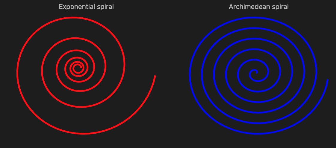
Raku has the built in mathematical constant  (base of the natural logarithm). Both ASCII “e” and Unicode “𝑒” (“MATHEMATICAL ITALIC SMALL E” or U+1D452) can be used:

[e, 𝑒]
# [2.718281828459045 2.718281828459045]

We can verify this famous equation:

e ** (i * π) + 1
# 0+1.2246467991473532e-16i

Let us compute  using the canonical formula:

Here is the corresponding Raku code:

my @e-terms = ([\*] 1.FatRat .. *);
my $e-by-sum = 1 + (1 «/» @e-terms[0 .. 100]).sum
# 2.7182818284590452353602874713526624977572470936999595749669676277240766303535475945713821785251664274274663919320030599218174135966290435729003342952605956307381312

Here we compute the e using Wolfram Language (via wolframscript):

my $proc = run 'wolframscript', '--code', 'N[E, 100]', :out;
my $e-wl = $proc.out.slurp(:close).substr(0,*-6).FatRat
# 2.7182818284590452353602874713526624977572470936999595749669676277240766303535475945713821785251664274274661651602106

Side-by-side comparison:

#% html
[
{lang => 'Raku', value => $e-by-sum.Str.substr(0,100)},
{lang => 'Wolfram Language', value => $e-wl.Str.substr(0,100)}
]
==> to-html(field-names => <lang value>, align => 'left')
langvalue
Raku2.71828182845904523536028747135266249775724709369995957496696762772407663035354759457138217852516642
Wolfram Language2.71828182845904523536028747135266249775724709369995957496696762772407663035354759457138217852516642

And here is the absolute difference:

abs($e-by-sum - $e-wl).Num
# 2.2677179245992183e-106

Let us next compute e using the continued fraction formula:

To make the corresponding continued fraction we first generate its sequence using Philippe Deléham formula for OEIS sequence A003417:

my @rec = 2, 1, 2, 1, 1, 4, 1, 1, -1 * * + 0 * * + 0 * * + 2 * * + 0 * * + 0 * * ... Inf;
@rec[^20]
# (2 1 2 1 1 4 1 1 6 1 1 8 1 1 10 1 1 12 1 1)

Here is a function that computes the continuous fraction formula:

sub e-by-cf(UInt:D $i) { @rec[^$i].reverse».FatRat.reduce({$^b + 1 / $^a}) }

Remark: A more generic continued fraction computation is given in the Raku entry for “Continued fraction”.

Let us compare all three results:

#% html
[
{lang => 'Raku', formula => 'sum', value => $e-by-sum.Str.substr(0,100)},
{lang => 'Raku', formula => 'cont. fraction', value => &e-by-cf(150).Str.substr(0,100)},
{lang => 'WL', formula => '-', value => $e-wl.Str.substr(0,100)}
]
==> to-html(field-names => <lang formula value>, align => 'left')
langformulavalue
Rakusum2.71828182845904523536028747135266249775724709369995957496696762772407663035354759457138217852516642
Rakucont. fraction2.71828182845904523536028747135266249775724709369995957496696762772407663035354759457138217852516642
WL2.71828182845904523536028747135266249775724709369995957496696762772407663035354759457138217852516642

Plots

The maximum of the function x^(1/x) is attained at e:

#% js
js-d3-list-line-plot((1, 1.01 ... 5).map({ [$_, $_ ** (1/$_)] }), :$background, stroke-width => 4, :grid-lines)

The Exponential spiral is based on the exponential function (and below it is compared to the Archimedean spiral):

#% js
my @log-spiral = (0, 0.1 ... 12 * π).map({ e ** ($_/12) «*» [cos($_), sin($_)] });
my @arch-spiral = (0, 0.1 ... 12 * π).map({ 2 * $_ «*» [cos($_), sin($_)] });
my %opts = stroke-width => 4, :!axes, :!grid-lines, :400width, :350height, :$title-color;
js-d3-list-line-plot(@log-spiral, :$background, color => 'red', title => 'Exponential spiral', |%opts) ~
js-d3-list-line-plot(@arch-spiral, :$background, color => 'blue', title => 'Archimedean spiral', |%opts)

Catenary is the curve a hanging flexible wire or chain assumes when supported at its ends and acted upon by a uniform gravitational force. It is given with the formula:

Here is a corresponding plot:

#% js
js-d3-list-line-plot((-1, -0.99 ... 1).map({ [$_, e ** $_ + e ** (-$_)] }), :$background, stroke-width => 4, :grid-lines, title => 'Catenary curve', :$title-color)

Fractals

The exponential curlicue fractal:

#%js
js-d3-list-line-plot(angle-path(e <<*>> (1...15_000)), :$background, :!axes, :400width, :600height)

Here is a plot of exponential Mandelbrot set:

my $h = 0.01;
my @table = do for -2.5, -2.5 + $h ... 2.5 -> $x {
do for -1, -1 + $h ... 4 -> $y {
my $z = 0;
my $count = 0;
while $count < 30 && $z.abs < 10e12 {
$z = exp($z) + $y + $x * i;
$count++;
}
$count - 1;
}
}
deduce-type(@table)
#% js
js-d3-matrix-plot(@table, :!grid-lines, color-palette => 'Rainbow', :!tooltip, :!mesh)

A fractal variant using reciprocal:

my $h = 0.0025;
my @table = do for -1/2, -1/2 + $h ... 1/6 -> $x {
do for -1/2, -1/2 + $h ... 1/2 -> $y {
my $z = $x + $y * i;
my $count = 0;
while $count < 10 && $z.abs < 100000 {
$z = exp(1 / $z);
$count++;
}
$count;
}
}
deduce-type(@table)
#% js
js-d3-matrix-plot(@table, :!grid-lines, color-palette => 'Rainbow', :!tooltip, :!mesh)

Data science over small movie dataset – Part 2

Introduction

This document (notebook) shows transformation of movie dataset into a form more suitable for making a movie recommender system. (It builds upon Part 1 of the blog posts series.)

The movie data was downloaded from “IMDB Movie Ratings Dataset”. That dataset was chosen because:

  • It has the right size for demonstration of data wrangling techniques
    • ≈5000 rows and 15 columns (each row corresponding to a movie)
  • It is “real life” data with expected skewness of variable distributions
  • It is diverse enough over movie years and genres
  • Relatively small number of missing values

The full “Raku for Data Science” showcase is done with three notebooks, [AAn1, AAn2, AAn3]:

  1. Data transformations and analysis, [AAn1]
  2. Sparse matrix recommender, [AAn2]
  3. Relationships graphs, [AAn3]

Remark: All three notebooks feature the same introduction, setup, and references sections in order to make it easier for readers to browse, access, or reproduce the content.

Remark: The series data files can be found in the folder “Data” of the GitHub repository “RakuForPrediction-blog”, [AAr1].

The notebook series can be used in several ways:

  • Just reading this introduction and then browsing the notebooks
  • Reading only this (data transformations) notebook in order to see how data wrangling is done
  • Evaluating all three notebooks in order to learn and reproduce the computational steps in them

Outline

Here are the transformation, data analysis, and machine learning steps taken in the notebook series, [AAn1, AAn2, AAn3]:

  1. Ingest the data — Part 1
    • Shape size and summaries
    • Numerical columns transformation
    • Renaming columns to have more convenient names
    • Separating the non-uniform genres column into movie-genre associations
      • Into long format
  2. Basic data analysis — Part 1
    • Number of movies per year distribution
    • Movie-genre distribution
    • Pareto principle adherence for movie directors
    • Correlation between number of votes and rating
  3. Association Rules Learning (ARL) — Part 1
    • Converting long format dataset into “baskets” of genres
    • Most frequent combinations of genres
    • Implications between genres
      • I.e. a biography-movie is also a drama-movie 94% of the time
    • LLM-derived dictionary of most commonly used ARL measures
  4. Recommender system creation — Part 2
    • Conversion of numerical data into categorical data
    • Application of one hot embedding
    • Experimenting / observing recommendation results
    • Getting familiar with the movie data by computing profiles for sets of movies
  5. Relationships graphs — Part 3
    • Find the nearest neighbors for every movie in a certain range of years
    • Make the corresponding nearest neighbors graph
      • Using different weights for the different types of movie metadata
    • Visualize largest components
    • Make and visualize graphs based on different filtering criteria

Comments & observations

  • This notebook series started as a demonstration of making a “real life” data Recommender System (RS).
    • The data transformations notebook would not be needed if the data had “nice” tabular form.
      • Since the data have aggregated values in its “genres” column typical long form transformations have to be done.
      • On the other hand, the actor names per movie are not aggregated but spread-out in three columns.
      • Both cases represent a single movie metadata type.
        • For both long format transformations (or similar) are needed in order to make an RS.
    • After a corresponding Sparse Matrix Recommender (SMR) is made its sparse matrix can be used to do additional analysis.
      • Such extensions are: deriving clusters, making and visualizing graphs, making and evaluating suitable classifiers.
  • In most “real life” data processing most of the data transformation listed steps above are taken.
  • ARL can be also used for deriving recommendations if the data is large enough.
  • The SMR object is based on Nearest Neighbors finding over “bags of tags.”
    • Latent Semantic Indexing (LSI) tag-weighting functions are applied.
  • The data does not have movie-viewer data, hence only item-item recommenders are created and used.
  • One hot embedding is a common technique, which in this notebook is done via cross-tabulation.
  • The categorization of numerical data means putting number into suitable bins or “buckets.”
    • The bin or bucket boundaries can be on a regular grid or a quantile grid.
  • For categorized numerical data one-hot embedding matrices can be processed to increase similarity between numeric buckets that are close to each to other.
  • Nearest-neighbors based recommenders — like SMR — can be used as classifiers.
    • These are the so called K-Nearest Neighbors (KNN) classifiers.
    • Although the data is small (both row-wise & column-wise) we can consider making classifiers predicting IMDB ratings or number of votes.
  • Using the recommender matrix similarities between different movies can be computed and a corresponding graph can be made.
  • Centrality analysis and simulations of random walks over the graph can be made.
    • Like Google’s “Page-rank” algorithm.
  • The relationship graphs can be used to visualize the “structure” of movie dataset.
  • Alternatively, clustering can be used.
    • Hierarchical clustering might be of interest.
  • If the movies had reviews or summaries associated with them, then Latent Semantic Analysis (LSA) could be applied.
    • SMR can use both LSA-terms-based and LSA-topics-based representations of the movies.
    • LLMs can be used to derive the LSA representation.
    • Again, not done in these series of notebooks.

Setup

Load packages used in the notebook:

use Math::SparseMatrix;
use ML::SparseMatrixRecommender;
use ML::SparseMatrixRecommender::Utilities;
use Statistics::OutlierIdentifiers;

#% javascript
require.config({
     paths: {
     d3: 'https://d3js.org/d3.v7.min'
}});

require(['d3'], function(d3) {
     console.log(d3);
});

#% js
js-d3-list-line-plot(10.rand xx 40, background => 'none', stroke-width => 2)

my $title-color = 'Silver';
my $stroke-color = 'SlateGray';
my $tooltip-color = 'LightBlue';
my $tooltip-background-color = 'none';
my $tick-labels-font-size = 10;
my $tick-labels-color = 'Silver';
my $tick-labels-font-family = 'Helvetica';
my $background = '#1F1F1F';
my $color-scheme = 'schemeTableau10';
my $color-palette = 'Inferno';
my $edge-thickness = 3;
my $vertex-size = 6;
my $mmd-theme = q:to/END/;
%%{
  init: {
    'theme': 'forest',
    'themeVariables': {
      'lineColor': 'Ivory'
    }
  }
}%%
END
my %force = collision => {iterations => 0, radius => 10},link => {distance => 180};
my %force2 = charge => {strength => -30, iterations => 4}, collision => {radius => 50, iterations => 4}, link => {distance => 30};

my %opts = :$background, :$title-color, :$edge-thickness, :$vertex-size;

# {background => #1F1F1F, edge-thickness => 3, title-color => Silver, vertex-size => 6}


Ingest data

Download from GitHub the files:

And unzip them.

Ingest movie data:

my $fileName = $*HOME ~ '/Downloads/movie_data.csv';
my @dsMovieData=data-import($fileName, headers=>'auto');
@dsMovieData .= map({ $_<title_year> = $_<title_year>.Int.Str; $_});
deduce-type(@dsMovieData)

# Vector(Assoc(Atom((Str)), Atom((Str)), 15), 5043)

Here is a sample of the movie data over the columns we most interested in:

#% html
my @movie-columns = <index movie_title title_year genres imdb_score num_voted_users>;
@dsMovieData.pick(4)
==> to-html(field-names => @movie-columns)

indexmovie_titletitle_yeargenresimdb_scorenum_voted_users
3322Veronika Decides to Die2009Drama|Romance6.510100
1511The Maze Runner2014Action|Mystery|Sci-Fi|Thriller6.8310903
1301Big Miracle2012Biography|Drama|Romance6.515231
55The Good Dinosaur2015Adventure|Animation|Comedy|Family|Fantasy6.862836

Ingest the movie data already transformed in the first notebook, [AAn1]:

my @dsMovieDataLongForm = data-import($*HOME ~ '/Downloads/dsMovieDataLongForm.csv', headers => 'auto');
deduce-type(@dsMovieDataLongForm)

# Vector(Assoc(Atom((Str)), Atom((Str)), 3), 84481)

Data summary:

my @field-names = <Item TagType Tag>;
sink records-summary(@dsMovieDataLongForm, :@field-names)

# +------------------+------------------------+-------------------+
# | Item             | TagType                | Tag               |
# +------------------+------------------------+-------------------+
# | 1387    => 27    | genre         => 29008 | Drama    => 5188  |
# | 3539    => 27    | actor         => 15129 | English  => 4704  |
# | 902     => 27    | title         => 5043  | USA      => 3807  |
# | 2340    => 27    | reviews_count => 5043  | Comedy   => 3744  |
# | 839     => 25    | language      => 5043  | Thriller => 2822  |
# | 1667    => 25    | country       => 5043  | Action   => 2306  |
# | 466     => 25    | director      => 5043  | Romance  => 2214  |
# | (Other) => 84298 | (Other)       => 15129 | (Other)  => 59696 |
# +------------------+------------------------+-------------------+


Recommender system

One way to investigate (browse) the data is to make a recommender system and explore with it different aspects of the movie dataset like movie profiles and nearest neighbors similarities distribution.

Make the recommender

In order to make a more meaningful recommender we put the values of the different numerical variables into “buckets” — i.e. intervals derived corresponding to the values distribution for each variable. The boundaries of the intervals can form a regular grid, correspond to quanitile values, or be specially made. Here we use quantiles:

my @bucketVars = <score votes_count reviews_count>;
my @dsMovieDataLongForm2;
sink for @dsMovieDataLongForm.map(*<TagType>).unique -> $var {
    if $var ∈ @bucketVars {
        my %bucketizer = ML::SparseMatrixRecommender::Utilities::categorize-to-intervals(@dsMovieDataLongForm.grep(*<TagType> eq $var).map(*<Tag>)».Numeric, probs => (0..6) >>/>> 6, :interval-names):pairs;
        @dsMovieDataLongForm2.append(@dsMovieDataLongForm.grep(*<TagType> eq $var).map(*.clone).map({ $_<Tag> = %bucketizer{$_<Tag>}; $_ }))
    } else {
        @dsMovieDataLongForm2.append(@dsMovieDataLongForm.grep(*<TagType> eq $var))
    }
}

sink records-summary(@dsMovieDataLongForm2, :@field-names, :12max-tallies)

# +------------------+------------------------+--------------------+
# | Item             | TagType                | Tag                |
# +------------------+------------------------+--------------------+
# | 902     => 19    | actor         => 15129 | English   => 4704  |
# | 2340    => 19    | genre         => 14504 | USA       => 3807  |
# | 1387    => 19    | score         => 5043  | Drama     => 2594  |
# | 3539    => 19    | country       => 5043  | Comedy    => 1872  |
# | 152     => 18    | votes_count   => 5043  | Thriller  => 1411  |
# | 466     => 18    | language      => 5043  | Action    => 1153  |
# | 1424    => 18    | year          => 5043  | Romance   => 1107  |
# | 839     => 18    | director      => 5043  | Adventure => 923   |
# | 132     => 18    | title         => 5043  | 6.1≤v<6.6 => 901   |
# | 113     => 18    | reviews_count => 5043  | 7≤v<7.5   => 891   |
# | 720     => 18    |                        | Crime     => 889   |
# | 1284    => 18    |                        | 7.5≤v<9.5 => 886   |
# | (Other) => 69757 |                        | (Other)   => 48839 |
# +------------------+------------------------+--------------------+


Here we make a Sparse Matrix Recommender (SMR):

my $smrObj = 
    ML::SparseMatrixRecommender.new
    .create-from-long-form(
        @dsMovieDataLongForm2, 
        item-column-name => 'Item', 
        tag-type-column-name => 'TagType',
        tag-column-name => 'Tag',
        :add-tag-types-to-column-names)        
    .apply-term-weight-functions('IDF', 'None', 'Cosine')

# ML::SparseMatrixRecommender(:matrix-dimensions((5043, 13825)), :density(<23319/23239825>), :tag-types(("reviews_count", "score", "votes_count", "genre", "country", "language", "actor", "director", "title", "year")))

Here are the recommender sub-matrices dimensions (rows and columns):

.say for $smrObj.take-matrices.deepmap(*.dimensions).sort(*.key)

# actor => (5043 6256)
# country => (5043 66)
# director => (5043 2399)
# genre => (5043 26)
# language => (5043 48)
# reviews_count => (5043 7)
# score => (5043 7)
# title => (5043 4917)
# votes_count => (5043 7)
# year => (5043 92)


Note that the sub-matrices of “reviews_count”, “score”, and “votes_count” have small number of columns, corresponding to the number probabilities specified when categorizing to intervals.

Enhance with one-hot embedding

my $mat = $smrObj.take-matrices<year>;

my $matUp = Math::SparseMatrix.new(
    diagonal => 1/2 xx ($mat.columns-count - 1), k => 1, 
    row-names => $mat.column-names,
    column-names => $mat.column-names
);

my $matDown = $matUp.transpose;

# mat = mat + mat . matDown + mat . matDown
$mat = $mat.add($mat.dot($matUp)).add($mat.dot($matDown));

# Math::SparseMatrix(:specified-elements(14915), :dimensions((5043, 92)), :density(<14915/463956>))

Make a new recommender with the enhanced matrices:

my %matrices = $smrObj.take-matrices;
%matrices<year> = $mat;
my $smrObj2 = ML::SparseMatrixRecommender.new(%matrices)

# ML::SparseMatrixRecommender(:matrix-dimensions((5043, 13825)), :density(<79829/69719475>), :tag-types(("genre", "title", "year", "actor", "director", "votes_count", "reviews_count", "score", "country", "language")))

Recommendations

Example recommendation by profile:

sink $smrObj2
.apply-tag-type-weights({genre => 2})
.recommend-by-profile(<genre:History year:1999>, 12, :!normalize)
.join-across(select-columns(@dsMovieData, @movie-columns), 'index')
.echo-value(as => {to-pretty-table($_, align => 'l', field-names => ['score', |@movie-columns])})

# +----------+-------+------------------------------------------+------------+----------------------------------------------+------------+-----------------+
# | score    | index | movie_title                              | title_year | genres                                       | imdb_score | num_voted_users |
# +----------+-------+------------------------------------------+------------+----------------------------------------------+------------+-----------------+
# | 1.887751 | 553   | Anna and the King                       | 1999       | Drama|History|Romance                        | 6.7        | 31080           |
# | 1.817476 | 215   | The 13th Warrior                        | 1999       | Action|Adventure|History                     | 6.6        | 101411          |
# | 1.567726 | 1016  | The Messenger: The Story of Joan of Arc | 1999       | Adventure|Biography|Drama|History|War        | 6.4        | 55889           |
# | 1.500264 | 2468  | One Man's Hero                          | 1999       | Action|Drama|History|Romance|War|Western     | 6.2        | 899             |
# | 1.487091 | 2308  | Topsy-Turvy                             | 1999       | Biography|Comedy|Drama|History|Music|Musical | 7.4        | 10037           |
# | 1.479006 | 4006  | La otra conquista                       | 1998       | Drama|History                                | 6.8        | 1024            |
# | 1.411933 | 492   | Thirteen Days                           | 2000       | Drama|History|Thriller                       | 7.3        | 45231           |
# | 1.312900 | 909   | Beloved                                 | 1998       | Drama|History|Horror                         | 5.9        | 6082            |
# | 1.237700 | 1931  | Elizabeth                               | 1998       | Biography|Drama|History                      | 7.5        | 75973           |
# | 1.168287 | 253   | The Patriot                             | 2000       | Action|Drama|History|War                     | 7.1        | 207613          |
# | 1.069476 | 1820  | The Newton Boys                         | 1998       | Action|Crime|Drama|History|Western           | 6.0        | 8309            |
# | 1.000000 | 4767  | America Is Still the Place              | 2015       | History                                      | 7.5        | 22              |
# +----------+-------+------------------------------------------+------------+----------------------------------------------+------------+-----------------+


Recommendation by history:

sink $smrObj
.recommend(<2125 2308>, 12, :!normalize, :!remove-history)
.join-across(select-columns(@dsMovieData, @movie-columns), 'index')
.echo-value(as => {to-pretty-table($_, align => 'l', field-names => ['score', |@movie-columns])})

# +-----------+-------+-------------------------+------------+----------------------------------------------+------------+-----------------+
# | score     | index | movie_title             | title_year | genres                                       | imdb_score | num_voted_users |
# +-----------+-------+-------------------------+------------+----------------------------------------------+------------+-----------------+
# | 12.510011 | 2125  | Molière                | 2007       | Comedy|History                               | 7.3        | 5166            |
# | 12.510011 | 2308  | Topsy-Turvy            | 1999       | Biography|Comedy|Drama|History|Music|Musical | 7.4        | 10037           |
# | 8.364831  | 1728  | The Color of Freedom   | 2007       | Biography|Drama|History                      | 7.1        | 10175           |
# | 8.182233  | 1724  | Little Nicholas        | 2009       | Comedy|Family                                | 7.2        | 9214            |
# | 7.753039  | 3619  | Little Voice           | 1998       | Comedy|Drama|Music|Romance                   | 7.0        | 13892           |
# | 7.439471  | 2285  | Mrs Henderson Presents | 2005       | Comedy|Drama|Music|War                       | 7.1        | 13505           |
# | 7.430299  | 3404  | Made in Dagenham       | 2010       | Biography|Comedy|Drama|History               | 7.2        | 11158           |
# | 7.270637  | 1799  | A Passage to India     | 1984       | Adventure|Drama|History                      | 7.4        | 12980           |
# | 7.264810  | 3837  | The Names of Love      | 2010       | Comedy|Drama|Romance                         | 7.2        | 6304            |
# | 7.117232  | 4648  | The Hammer             | 2007       | Comedy|Romance|Sport                         | 7.3        | 5489            |
# | 7.046925  | 4871  | Shotgun Stories        | 2007       | Drama|Thriller                               | 7.3        | 7148            |
# | 7.040720  | 3194  | The House of Mirth     | 2000       | Drama|Romance                                | 7.1        | 6377            |
# +-----------+-------+-------------------------+------------+----------------------------------------------+------------+-----------------+


Profiles

Find movie IDs for a certain criteria (e.g. historic action movies):

my @movieIDs = $smrObj.recommend-by-profile(<genre:Action genre:History>, Inf, :!normalize).take-value.grep(*.value > 1)».key;
deduce-type(@movieIDs)

# Vector(Atom((Str)), 14)

Find the profile of the movie set:

my @profile = |$smrObj.profile(@movieIDs).take-value;
deduce-type(@profile)

# Vector(Pair(Atom((Str)), Atom((Numeric))), 108)

Find the top outliers in that profile:

outlier-identifier(@profile».value, identifier => &top-outliers o &quartile-identifier-parameters)
==> {@profile[$_]}()
==> my @profile2;

deduce-type(@profile2)

# Vector(Pair(Atom((Str)), Atom((Numeric))), 26)

Here is a table of the top outlier profile tags and their scores:

#%html
@profile.head(28)
==> { $_.map({ to-html-table([$_,]) }) }()
==> to-html(:multi-column, :4columns, :html-elements)

genre:History0.9999999999999999language:Mandarin0.3626315299347615score:7.5≤v<9.50.2719736474510711year:20150.18131576496738075
language:English0.8159209423532133reviews_count:0≤v<370.3626315299347615votes_count:5≤v<41200.2719736474510711year:20140.18131576496738075
genre:Action0.46214109363846967score:6.1≤v<6.60.36263152993476144title:Hero0.18131576496738075country:UK0.18131576496738075
genre:Adventure0.38097093240387203country:USA0.36263152993476144votes_count:68935≤v<1473170.18131576496738075score:7≤v<7.50.18131576496738075
score:6.6≤v<70.3626315299347615reviews_count:450≤v<50600.36263152993476144reviews_count:37≤v<910.18131576496738075votes_count:4120≤v<149850.18131576496738072
country:China0.3626315299347615votes_count:147317≤v<16897640.2719736474510711year:20020.18131576496738075genre:Drama0.1320986315690731
votes_count:14985≤v<343590.3626315299347615reviews_count:91≤v<1550.2719736474510711director:Yimou Zhang0.18131576496738075genre:Romance0.13001981085966202

Plot all of profile’s scores and the score outliers:

#%js
js-d3-list-plot(
    [|@profile».value.kv.map(-> $x, $y { %(:$x, :$y, group => 'full profile' ) }), 
     |@profile2».value.kv.map(-> $x, $y { %(:$x, :$y, group => 'outliers' ) })], 
    :$background,
    :300height,
    :600width
    )


References

Articles, blog posts

[AA1] Anton Antonov, “Introduction to data wrangling with Raku”, (2021), RakuForPrediction at WordPress.

[AA2] Anton Antonov, “Implementing Machine Learning algorithms in Raku (TRC-2022 talk)”, (2021), RakuForPrediction at WordPress.

Notebooks

[AAn1] Anton Antonov,
“Small movie dataset analysis”,
(2025),
RakuForPrediction-blog at GitHub.

[AAn2] Anton Antonov,
“Small movie dataset recommender”,
(2025),
RakuForPrediction-blog at GitHub.

[AAn3] Anton Antonov,
“Small movie dataset graph”,
(2025),
RakuForPrediction-blog at GitHub.

Packages

[AAp1] Anton Antonov, Data::Importers, Raku package, (2024-2025), GitHub/antononcube.

[AAp2] Anton Antonov, Data::Reshapers, Raku package, (2021-2025), GitHub/antononcube.

[AAp3] Anton Antonov, Data::Summarizers, Raku package, (2021-2024), GitHub/antononcube.

[AAp4] Anton Antonov, Graph, Raku package, (2024-2025), GitHub/antononcube.

[AAp5] Anton Antonov, JavaScript::D3, Raku package, (2022-2025), GitHub/antononcube.

[AAp6] Anton Antonov, Jupyter::Chatbook, Raku package, (2023-2025), GitHub/antononcube.

[AAp7] Anton Antonov, Math::SparseMatrix, Raku package, (2024-2025), GitHub/antononcube.

[AAp8] Anton Antonov, ML::AssociationRuleLearning, Raku package, (2022-2024), GitHub/antononcube.

[AAp9] Anton Antonov, ML::SparseMatrixRecommender, Raku package, (2025), GitHub/antononcube.

[AAp10] Anton Antonov, Statistics::OutlierIdentifiers, Raku package, (2022), GitHub/antononcube.

Videos

[AAv1] Anton Antonov, “Simplified Machine Learning Workflows Overview (Raku-centric)”, (2022), YouTube/@AAA4prediction.

[AAv2] Anton Antonov, “TRC 2022 Implementation of ML algorithms in Raku”, (2022), YouTube/@AAA4prediction.

[AAv3] Anton Antonov, “Exploratory Data Analysis with Raku”, (2024), YouTube/@AAA4prediction.

[AAv4] Anton Antonov, “Raku RAG demo”, (2024), YouTube/@AAA4prediction.

Graph::RandomMaze examples

Introduction

This document (notebook) demonstrates the functions of “Graph::RandomMaze”, [AAp1], for generating and displaying random mazes. The methodology and implementations of maze creation based on random rectangular and hexagonal grid graphs are described in detail in the blog post “Day 24 – Maze Making Using Graphs”, [AA1], and in the Wolfram notebook “Maze Making Using Graphs”, [AAn1].

Remark: The corresponding Wolfram Language implementation is Wolfram Function Repository function “RandomLabyrinth”, [AAf1].

Remark: Both synonyms, “labyrinth” and “maze,” are used in this document.

TL;DR

Just look at the “neat examples” in the last section.


Documentation

This section gives basic documentation of the subs.

Usage

FunctionDescription
random-maze(n)generate a random labyrinth based on n × n grid graph
random-maze([n, m])generate a random labyrinth based on a grid graph with n rows and m columns
&random-labyrintha synonym of &random-maze
display-maze(m)displays outputs random-maze using Graphviz graph layout engines

Details & Options

  • The sub random-maze generates mazes based on regular rectangular grid graphs or hexagonal grid graphs.
  • By default, are generated random mazes based on rectangular grid graphs.
  • The named argument (option) “type” can be used the specify the type of the grid graph used for maze’s construction.
  • The labyrinth elements can be obtained by using the second argument (the “properties argument.”)
  • The labyrinth elements are: walls, paths (pathways), solution, start, and end.
  • The sub display-maze can be used to make SVG images of the outputs of random-maze.
  • By default display-maze uses the Graphviz engine “neato”.
  • The sub random-maze uses the grid graphs Graph::GridGraph::HexagonalGrid, and Graph::TriangularGrid. For more details see [AA1, AAn1].
  • For larger sizes the maze generation might be (somewhat) slow.

Setup

Here are the packages used in this document:

use Graph::RandomMaze;
use Data::Generators;
use JavaScript::D3;
use Hash::Merge;

Here are Graph.dot options used in this document:

my $engine = 'neato';
my $vertex-shape = 'square';
my $graph-size = 8;
my %opts = :$engine, :8size, vertex-shape => 'square', :!vertex-labels, edge-thickness => 12;
my %hex-opts = :$engine, :8size, vertex-shape => 'hexagon', :!vertex-labels, vertex-width => 0.8, vertex-height => 0.8, edge-thickness => 32;

my $background = '#1F1F1F';

This code is used to prime the notebook to display (JavaScript) D3.js graphics:

#% javascript
require.config({
     paths: {
     d3: 'https://d3js.org/d3.v7.min'
}});

require(['d3'], function(d3) {
     console.log(d3);
});


Examples

Basic Examples

Make a random rectangular grid labyrinth with 8 rows and columns:

#%html
random-maze(8).dot(|%opts, :3size):svg

Make a random rectangular grid labyrinth with 5 rows and 8 columns:

#%html
random-maze([5, 8]).dot(|%opts, :3size):svg

Scope

Make a random hexagonal grid labyrinth:

#% html
random-maze([8, 16], type => "hexagonal").dot(|%hex-opts):svg

Make a labyrinth using options to specify the rows and columns of the walls graph:

#% html
random-maze(:10rows, :5columns)
andthen display-maze($_, |%opts, :3size)

The sub random-maze take an optional properties argument. Here are the different properties:

random-maze("properties")

# [type dimensions walls paths solution start end]

If the properties argument is Whatever, then an association with all properties is returned (“props” can be used instead of “properties”):

random-maze(5, props => Whatever)

# {dimensions => [5 5], end => 3_3, paths => Graph(vertexes => 16, edges => 15, directed => False), solution => [0_0 1_0 1_1 2_1 2_2 2_3 3_3], start => 0_0, type => rectangular, walls => Graph(vertexes => 23, edges => 21, directed => False)}

The first argument of the sub display-maze can be a graphs or a hashmap. Here is example of using both argument types:

#%html
my %new-opts = merge-hash(%opts, {:2size});
[
    graph   => display-maze(random-maze(5, props => 'walls' ), |%new-opts),
    hashmap => display-maze(random-maze(5, props => Whatever), |%new-opts) 
]
==> to-html-table()


Options

Type

The option :$type specifies the type grid graphs used to make the labyrinth. It takes the values “rectangular” and “hexagonal”:

#% html
<rectangular hexagonal>
andthen .map({ random-maze(7, type => $_, props => Whatever) }).List
andthen 
    [
        $_.head<type> => display-maze($_.head, |merge-hash(%opts, {:3size})), 
        $_.tail<type> => display-maze($_.tail, |merge-hash(%hex-opts, {size => 4.5}))
    ]
andthen .&to-html-table

DOT options

The sub display-graph takes Graphviz DOT options for more tuned maze display. The options are the same as those of Graph.dot.

#%html
random-maze([5, 10], props => 'walls')
==> display-maze(:$engine, vertex-shape => 'ellipse', vertex-width => 0.6, :6size)


Applications

Rectangular maze with solution

Make a rectangular grid labyrinth and show it together with a (shortest path) solution:

#%html
my %res = random-maze([12, 24], props => <walls paths solution>);

display-maze(%res, |%opts)

Hexagonal maze with solution

Make a hexagonal grid labyrinth and show it together with a (shortest path) solution:

#%html
my %res = random-maze([12, 20], type => 'hexagonal', props => <walls paths solution>);

display-maze(%res, |%hex-opts)

Distribution of solution lengths

Generate — in parallel — 500 mazes:

my @labs = (^500).race(:4degree, :125batch).map({ random-maze(12, props => <walls paths solution>) });
deduce-type(@labs)

# Vector(Struct([paths, solution, walls], [Graph, Array, Graph]), 500)

Show the histogram of the shortest path solution lengths:

#% js
js-d3-histogram(
    @labs.map(*<solution>)».elems, 
    title => 'Distribution of solution lengths',
    title-color => 'Silver',
    x-axis-label => 'shortest path solution length',
    y-axis-label => 'count',
    :$background, :grid-lines, 
    :350height, :450width
)

Show the mazes with the shortest and longest shortest paths solutions:

#% html
@labs.sort(*<solution>.elems).List
andthen 
    [
        "shortest : {$_.head<solution>.elems}" => display-maze($_.head, |merge-hash(%opts , {:3size})),
        "longest : {$_.tail<solution>.elems}"  => display-maze($_.tail, |merge-hash(%opts , {size => 3}))
    ]
andthen .&to-html-table


Neat Examples

Larger rectangular grid maze:

#%html
random-maze([30, 60]).dot(|%opts, edge-thickness => 25):svg

A larger hexagonal grid maze with its largest connected components colored:

#%html
my $g = random-maze([20, 30], type => 'hexagonal', props => 'walls');
$g.dot(highlight => $g.connected-components.head(2).map({ my $sg = $g.subgraph($_); [|$sg.vertex-list, |$sg.edge-list] }), |%hex-opts):svg

A grid of tiny labyrinths:

#%html
my $k = 6;
my @mazes = random-maze((6...7).pick) xx $k ** 2;
my %new-opts = size => 0.8, vertex-shape => 'circle', vertex-width => 0.35, vertex-height => 0.35, edge-thickness => 36;
my @maze-plots = @mazes.map({ $_.dot(|%opts, |%new-opts, :svg) });

@maze-plots
==> to-html(:multi-column, :6columns, :html-elements)


References

Articles

[AA1] Anton Antonov, “Day 24 – Maze Making Using Graphs”, (2025), Raku Advent Calendar at WordPress.

Notebooks

[AAn1] Anton Antonov, “Maze making using graphs”, (2026), Wolfram Community.

Functions, packages

[AAf1] Anton Antonov, RandomLabyrinth, (2025), Wolfram Function Repository.

[AAp1] Anton Antonov, Graph::RandomMaze, Raku package, (2025), GitHub/antononcube.

[AAp2] Anton Antonov, Graph, Raku package, (2024-2025), GitHub/antononcube.

Data science over small movie dataset — Part 1

«Data transformations and analysis»

Introduction

This document (notebook) shows transformations of a movie dataset into a format more suitable for data analysis and for making a movie recommender system. It is the first of a three-part series of notebooks that showcase Raku packages for doing Data Science (DS). The notebook series as a whole goes through this general DS loop:

The movie data was downloaded from “IMDB Movie Ratings Dataset”. That dataset was chosen because:

  • It has the right size for demonstration of data wrangling techniques
    • ≈5000 rows and 15 columns (each row corresponding to a movie)
  • It is “real life” data with expected skewness of variable distributions
  • It is diverse enough over movie years and genres
  • Relatively small number of missing values

The full “Raku for Data Science” showcase is done with three notebooks, [AAn1, AAn2, AAn3]:

  1. Data transformations and analysis, [AAn1]
  2. Sparse matrix recommender, [AAn2]
  3. Relationships graphs, [AAn3]

Remark: All three notebooks feature the same introduction, setup, and references sections in order to make it easier for readers to browse, access, or reproduce the content.

Remark: The series data files can be found in the folder “Data” of the GitHub repository “RakuForPrediction-blog”, [AAr1].

The notebook series can be used in several ways:

  • Just reading this introduction and then browsing the notebooks
  • Reading only this (data transformations) notebook in order to see how data wrangling is done
  • Evaluating all three notebooks in order to learn and reproduce the computational steps in them

Outline

Here are the transformation, data analysis, and machine learning steps taken in the notebook series, [AAn1, AAn2, AAn3]:

  1. Ingest the data — Part 1
    • Shape size and summaries
    • Numerical columns transformation
    • Renaming columns to have more convenient names
    • Separating the non-uniform genres column into movie-genre associations
      • Into long format
  2. Basic data analysis — Part 1
    • Number of movies per year distribution
    • Movie-genre distribution
    • Pareto principle adherence for movie directors
    • Correlation between number of votes and rating
  3. Association Rules Learning (ARL) — Part 1
    • Converting long format dataset into “baskets” of genres
    • Most frequent combinations of genres
    • Implications between genres
      • I.e. a biography-movie is also a drama-movie 94% of the time
    • LLM-derived dictionary of most commonly used ARL measures
  4. Recommender system creation — Part 2
    • Conversion of numerical data into categorical data
    • Application of one hot embedding
    • Experimenting / observing recommendation results
    • Getting familiar with the movie data by computing profiles for sets of movies
  5. Relationships graphs — Part 3
    • Find the nearest neighbors for every movie in a certain range of years
    • Make the corresponding nearest neighbors graph
      • Using different weights for the different types of movie metadata
    • Visualize largest components
    • Make and visualize graphs based on different filtering criteria

Comments & observations

  • This notebook series started as a demonstration of making a “real life” data Recommender System (RS).
    • The data transformations notebook would not be needed if the data had “nice” tabular form.
      • Since the data have aggregated values in its “genres” column typical long form transformations have to be done.
      • On the other hand, the actor names per movie are not aggregated but spread-out in three columns.
      • Both cases represent a single movie metadata type.
        • For both long format transformations (or similar) are needed in order to make an RS.
    • After a corresponding Sparse Matrix Recommender (SMR) is made its sparse matrix can be used to do additional analysis.
      • Such extensions are: deriving clusters, making and visualizing graphs, making and evaluating suitable classifiers.
  • In most “real life” data processing most of the data transformation listed steps above are taken.
  • ARL can be also used for deriving recommendations if the data is large enough.
  • The SMR object is based on Nearest Neighbors finding over “bags of tags.”
    • Latent Semantic Indexing (LSI) tag-weighting functions are applied.
  • The data does not have movie-viewer data, hence only item-item recommenders are created and used.
  • One hot embedding is a common technique, which in this notebook is done via cross-tabulation.
  • The categorization of numerical data means putting number into suitable bins or “buckets.”
    • The bin or bucket boundaries can be on a regular grid or a quantile grid.
  • For categorized numerical data one-hot embedding matrices can be processed to increase similarity between numeric buckets that are close to each to other.
  • Nearest-neighbors based recommenders — like SMR — can be used as classifiers.
    • These are the so called K-Nearest Neighbors (KNN) classifiers.
    • Although the data is small (both row-wise & column-wise) we can consider making classifiers predicting IMDB ratings or number of votes.
  • Using the recommender matrix similarities between different movies can be computed and a corresponding graph can be made.
  • Centrality analysis and simulations of random walks over the graph can be made.
    • Like Google’s “Page-rank” algorithm.
  • The relationship graphs can be used to visualize the “structure” of movie dataset.
  • Alternatively, clustering can be used.
    • Hierarchical clustering might be of interest.
  • If the movies had reviews or summaries associated with them, then Latent Semantic Analysis (LSA) could be applied.
    • SMR can use both LSA-terms-based and LSA-topics-based representations of the movies.
    • LLMs can be used to derive the LSA representation.
    • Again, not done in these series of notebooks.

Setup

Load packages used in the notebook:

use Math::SparseMatrix;
use ML::SparseMatrixRecommender;
use ML::SparseMatrixRecommender::Utilities;
use Statistics::OutlierIdentifiers;

Prime the notebook to show JavaScript plots:

#% javascript
require.config({
     paths: {
     d3: 'https://d3js.org/d3.v7.min'
}});

require(['d3'], function(d3) {
     console.log(d3);
});

Example JavaScript plot:

#% js
js-d3-list-line-plot(10.rand xx 40, background => 'none', stroke-width => 2)

Set different plot style variables:

my $title-color = 'Silver';
my $stroke-color = 'SlateGray';
my $tooltip-color = 'LightBlue';
my $tooltip-background-color = 'none';
my $tick-labels-font-size = 10;
my $tick-labels-color = 'Silver';
my $tick-labels-font-family = 'Helvetica';
my $background = 'White'; #'#1F1F1F';
my $color-scheme = 'schemeTableau10';
my $color-palette = 'Inferno';
my $edge-thickness = 3;
my $vertex-size = 6;
my $mmd-theme = q:to/END/;
%%{
  init: {
    'theme': 'forest',
    'themeVariables': {
      'lineColor': 'Ivory'
    }
  }
}%%
END
my %force = collision => {iterations => 0, radius => 10},link => {distance => 180};
my %force2 = charge => {strength => -30, iterations => 4}, collision => {radius => 50, iterations => 4}, link => {distance => 30};

sink my %opts = :$background, :$title-color, :$edge-thickness, :$vertex-size;


Ingest data

Ingest the movie data:

# Download and unzip: https://github.com/antononcube/RakuForPrediction-blog/raw/refs/heads/main/Data/movie_data.csv.zip
my $fileName=$*HOME ~ '/Downloads/movie_data.csv';
my @dsMovieData=data-import($fileName, headers=>'auto');

deduce-type(@dsMovieData)

# Vector(Assoc(Atom((Str)), Atom((Str)), 15), 5043)

Show a sample of the movie data:

#% html
my @field-names = <index movie_title title_year country duration language actor_1_name actor_2_name actor_3_name director_name imdb_score num_user_for_reviews num_voted_users movie_imdb_link>;
@dsMovieData.pick(8)
==> to-html(:@field-names)

Convert string values of the numerical columns into numbers:

@dsMovieData .= map({ 
    $_<title_year> = $_<title_year>.trim.Int; 
    $_<imdb_score> = $_<imdb_score>.Numeric; 
    $_<num_user_for_reviews> = $_<num_user_for_reviews>.Int; 
    $_<num_voted_users> = $_<num_voted_users>.Int; 
    $_});
deduce-type(@dsMovieData)

# Vector(Struct([actor_1_name, actor_2_name, actor_3_name, country, director_name, duration, genres, imdb_score, index, language, movie_imdb_link, movie_title, num_user_for_reviews, num_voted_users, title_year], [Str, Str, Str, Str, Str, Str, Str, Rat, Str, Str, Str, Str, Int, Int, Int]), 5043)

Summary of the numerical columns:

sink 
<index title_year imdb_score num_voted_users num_user_for_reviews>
andthen [select-columns(@dsMovieData, $_), $_]
andthen records-summary($_.head, field-names => $_.tail);

+-----------------+-----------------------+--------------------+------------------------+----------------------+
| index           | title_year            | imdb_score         | num_voted_users        | num_user_for_reviews |
+-----------------+-----------------------+--------------------+------------------------+----------------------+
| 252     => 1    | Min    => 0           | Min    => 1.6      | Min    => 5            | Min    => 0          |
| 1453    => 1    | 1st-Qu => 1998        | 1st-Qu => 5.8      | 1st-Qu => 8589         | 1st-Qu => 64         |
| 2004    => 1    | Mean   => 1959.585961 | Mean   => 6.442138 | Mean   => 83668.160817 | Mean   => 271.63494  |
| 3545    => 1    | Median => 2005        | Median => 6.6      | Median => 34359        | Median => 155        |
| 2903    => 1    | 3rd-Qu => 2011        | 3rd-Qu => 7.2      | 3rd-Qu => 96385        | 3rd-Qu => 324        |
| 2429    => 1    | Max    => 2016        | Max    => 9.5      | Max    => 1689764      | Max    => 5060       |
| 2764    => 1    |                       |                    |                        |                      |
| (Other) => 5036 |                       |                    |                        |                      |
+-----------------+-----------------------+--------------------+------------------------+----------------------+

Summary of the name-columns in the data:

sink 
<director_name actor_1_name actor_2_name actor_3_name>
andthen [select-columns(@dsMovieData, $_), $_]
andthen records-summary($_.head, field-names => $_.tail);

+--------------------------+---------------------------+-------------------------+------------------------+
| director_name            | actor_1_name              | actor_2_name            | actor_3_name           |
+--------------------------+---------------------------+-------------------------+------------------------+
|                  => 104  | Robert De Niro    => 49   | Morgan Freeman  => 20   |                => 23   |
| Steven Spielberg => 26   | Johnny Depp       => 41   | Charlize Theron => 15   | Steve Coogan   => 8    |
| Woody Allen      => 22   | Nicolas Cage      => 33   | Brad Pitt       => 14   | John Heard     => 8    |
| Clint Eastwood   => 20   | J.K. Simmons      => 31   |                 => 13   | Ben Mendelsohn => 8    |
| Martin Scorsese  => 20   | Denzel Washington => 30   | Meryl Streep    => 11   | Anne Hathaway  => 7    |
| Ridley Scott     => 17   | Bruce Willis      => 30   | James Franco    => 11   | Stephen Root   => 7    |
| Spike Lee        => 16   | Matt Damon        => 30   | Jason Flemyng   => 10   | Sam Shepard    => 7    |
| (Other)          => 4818 | (Other)           => 4799 | (Other)         => 4949 | (Other)        => 4975 |
+--------------------------+---------------------------+-------------------------+------------------------+

Convert to long form by skipping special columns (like “genres”):

my @varnames = <movie_title title_year country actor_1_name actor_2_name actor_3_name num_voted_users num_user_for_reviews imdb_score director_name language>;
my @dsMovieDataLongForm = to-long-format(@dsMovieData, 'index', @varnames, variables-to => 'TagType', values-to => 'Tag');

deduce-type(@dsMovieDataLongForm)

#  Vector((Any), 55473)

Remark: The transformation above is also known as “unpivoting” or “pivoting columns into rows”.

Show a sample of the converted data:

#% html
@dsMovieDataLongForm.pick(8)
==> to-html(field-names => <index TagType Tag>)

indexTagTypeTag
3586title_year1980
539actor_3_nameBen Mendelsohn
1087countryUSA
968languageEnglish
4856director_nameMaria Maggenti
3101movie_titleThe Longest Day 
2297num_user_for_reviews26
684num_user_for_reviews175

Give some tag types more convenient names:

my %toBetterTagTypes = 
    movie_title => 'title', 
    title_year => 'year', 
    director_name => 'director',
    actor_1_name => 'actor', actor_2_name => 'actor', actor_3_name => 'actor', 
    num_voted_users => 'votes_count', num_user_for_reviews => 'reviews_count',
    imdb_score => 'score', 
    ;

@dsMovieDataLongForm = @dsMovieDataLongForm.map({ $_<TagType> = %toBetterTagTypes{$_<TagType>} // $_<TagType>; $_ });
@dsMovieDataLongForm = |rename-columns(@dsMovieDataLongForm, {index=>'Item'});

deduce-type(@dsMovieDataLongForm)

# Vector((Any), 55473)

Summarize the long form data:

sink records-summary(@dsMovieDataLongForm, :12max-tallies)

+------------------------+------------------+------------------+
| TagType                | Tag              | Item             |
+------------------------+------------------+------------------+
| actor         => 15129 | English => 4704  | 4173    => 11    |
| title         => 5043  | USA     => 3807  | 1330    => 11    |
| votes_count   => 5043  | UK      => 448   | 552     => 11    |
| reviews_count => 5043  | 2009    => 260   | 5022    => 11    |
| country       => 5043  | 2014    => 252   | 4503    => 11    |
| language      => 5043  | 2006    => 239   | 463     => 11    |
| year          => 5043  | 2013    => 237   | 395     => 11    |
| score         => 5043  | 2010    => 230   | 3122    => 11    |
| director      => 5043  | 2015    => 226   | 4873    => 11    |
|                        | 2011    => 226   | 2959    => 11    |
|                        | 2008    => 225   | 23      => 11    |
|                        | 2012    => 223   | 715     => 11    |
|                        | (Other) => 44396 | (Other) => 55341 |
+------------------------+------------------+------------------+

Make a separate dataset with movie-genre associations:

my @dsMovieGenreLongForm = @dsMovieData.map({ $_<index> X $_<genres>.split('|', :skip-empty)}).flat(1).map({ <index genre> Z=> $_ })».Hash;
deduce-type(@dsMovieGenreLongForm)

# Vector(Assoc(Atom((Str)), Atom((Str)), 2), 14504)

Make the genres long form similar to that with the rest of the movie metadata:

@dsMovieGenreLongForm = rename-columns(@dsMovieGenreLongForm, {index => 'Item', genre => 'Tag'}).map({ $_.push('TagType' => 'genre') });

deduce-type(@dsMovieGenreLongForm)

# Vector(Assoc(Atom((Str)), Atom((Str)), 3), 14504)

#% html
@dsMovieGenreLongForm.head(8)
==> to-html(field-names => <Item TagType Tag>)

ItemTagTypeTag
0genreAction
0genreAdventure
0genreFantasy
0genreSci-Fi
1genreAction
1genreAdventure
1genreFantasy
2genreAction

Statistics

In this section we compute different statistics that should give us better idea what the data is.

Show movie years distribution:

#% js
js-d3-bar-chart(@dsMovieData.map(*<title_year>.Str).&tally.sort(*.head), title => 'Movie years distribution', :$title-color, :1200width, :$background)
~
js-d3-box-whisker-chart(@dsMovieData.map(*<title_year>)».Int.grep(*>1916), :horizontal, :$background)

Show movie genre distribution:

#% js
my %genreCounts = cross-tabulate(@dsMovieGenreLongForm, 'Item', 'Tag', :sparse).column-sums(:p);
js-d3-bar-chart(%genreCounts.sort, title => 'Genre distributions', :$background, :$title-color)

Check Pareto principle adherence for director names:

#% js
pareto-principle-statistic(@dsMovieData.map(*<director_name>))
==> js-d3-list-line-plot(
        :$background,
        title => 'Pareto principle adherence for movie directors',
        y-label => 'probability', x-label => 'index',
        :grid-lines, :5stroke-width, :$title-color)

Plot the number of IMDB votes vs IMBDB scores:

#% js
@dsMovieData.map({ %( x => $_<num_voted_users>».Num».log(10), y => $_<imdb_score>».Num ) })
==> js-d3-list-plot(
        :$background,
        title => 'Number of IMBD votes vs IMDB scores',
        x-label => 'Number of votes, lg', y-label => 'score',
        :grid-lines, point-size => 4, :$title-color)


Association rules learning

It is interesting to see which genres associated closely with each other. One way to find to those associations is to use Association Rule Learning (ARL).

For each movie make a “basket” of genres:

my @baskets = cross-tabulate(@dsMovieGenreLongForm, 'Item', 'Tag').values».keys».List;
@baskets».elems.&tally

# {1 => 633, 2 => 1355, 3 => 1628, 4 => 981, 5 => 349, 6 => 75, 7 => 18, 8 => 4}

Find frequent sets that are seen in at least 300 movies:

my @freqSets = frequent-sets(@baskets, min-support => 300, min-number-of-items => 2, max-number-of-items => Inf);
deduce-type(@freqSets):tally

# Tuple([Pair(Vector(Atom((Str)), 2), Atom((Rat))) => 14, Pair(Vector(Atom((Str)), 3), Atom((Rat))) => 1], 15)

to-pretty-table(@freqSets.map({ %( FrequentSet => $_.key.join(' '), Frequency => $_.value) }).sort(-*<Frequency>), field-names => <FrequentSet Frequency>, align => 'l');

+----------------------+-----------+
| FrequentSet          | Frequency |
+----------------------+-----------+
| Drama Romance        | 0.146143  |
| Drama Thriller       | 0.138211  |
| Comedy Drama         | 0.131469  |
| Action Thriller      | 0.116796  |
| Comedy Romance       | 0.116796  |
| Crime Thriller       | 0.108665  |
| Crime Drama          | 0.104303  |
| Action Adventure     | 0.093198  |
| Comedy Family        | 0.070989  |
| Mystery Thriller     | 0.070196  |
| Action Drama         | 0.068412  |
| Action Sci-Fi        | 0.066627  |
| Crime Drama Thriller | 0.066032  |
| Action Crime         | 0.065041  |
| Adventure Comedy     | 0.061670  |
+----------------------+-----------+

Here are the corresponding association rules:

association-rules(@baskets, min-support => 0.025, min-confidence => 0.70)
==> { .sort(-*<confidence>) }()
==> { to-pretty-table($_, field-names => <antecedent consequent count support confidence lift leverage conviction>) }()

+---------------------+------------+-------+----------+------------+----------+----------+------------+
|      antecedent     | consequent | count | support  | confidence |   lift   | leverage | conviction |
+---------------------+------------+-------+----------+------------+----------+----------+------------+
|      Biography      |   Drama    |  275  | 0.054531 |  0.938567  | 1.824669 | 0.024646 |  7.904874  |
|       History       |   Drama    |  189  | 0.037478 |  0.913043  | 1.775049 | 0.016364 |  5.584672  |
|   Animation Comedy  |   Family   |  154  | 0.030537 |  0.895349  | 8.269678 | 0.026845 |  8.520986  |
| Adventure Animation |   Family   |  151  | 0.029942 |  0.893491  | 8.252520 | 0.026314 |  8.372364  |
|         War         |   Drama    |  190  | 0.037676 |  0.892019  | 1.734175 | 0.015950 |  4.497297  |
|      Animation      |   Family   |  205  | 0.040650 |  0.847107  | 7.824108 | 0.035455 |  5.832403  |
|    Crime Mystery    |  Thriller  |  129  | 0.025580 |  0.821656  | 2.936649 | 0.016869 |  4.038299  |
|     Action Crime    |  Thriller  |  259  | 0.051358 |  0.789634  | 2.822201 | 0.033160 |  3.423589  |
|  Adventure Thriller |   Action   |  175  | 0.034702 |  0.781250  | 3.417037 | 0.024546 |  3.526246  |
|    Drama Mystery    |  Thriller  |  200  | 0.039659 |  0.769231  | 2.749278 | 0.025234 |  3.120894  |
|   Animation Family  |   Comedy   |  154  | 0.030537 |  0.751220  | 2.023718 | 0.015448 |  2.527499  |
|   Adventure Sci-Fi  |   Action   |  193  | 0.038271 |  0.736641  | 3.221927 | 0.026393 |  2.928956  |
|   Animation Family  | Adventure  |  151  | 0.029942 |  0.736585  | 4.024485 | 0.022502 |  3.101475  |
|      Animation      |   Comedy   |  172  | 0.034107 |  0.710744  | 1.914680 | 0.016293 |  2.173825  |
|       Mystery       |  Thriller  |  354  | 0.070196 |  0.708000  | 2.530435 | 0.042456 |  2.466460  |
+---------------------+------------+-------+----------+------------+----------+----------+------------+

Measure cheat-sheet

Here is a table showing the formulas for the Association Rules Learning measures (confidence, lift, leverage, conviction), along with their minimum value, maximum value, and value of indifference:

Explanation of terms:

  • support(X) = P(X), the proportion of transactions containing itemset X.
  • ¬A = complement of A (transactions not containing A).
  • Value of indifference generally means the value where the measure indicates independence or no association.
  • For Confidence, the baseline is support(B) (probability of B alone).
  • For Lift and Conviction, 1 indicates no association.
  • Leverage’s minimum and maximum depend on the supports of A and B.

LLM prompt

Here is the prompt used to generate the ARL metrics dictionary table above:

Give the formulas for the Association Rules Learning measures: confidence, lift, leverage, and conviction.
In a Markdown table for each measure give the min value, max value, value of indifference. Make sure the formulas are in LaTeX code.


Export transformed data

Here we export the transformed data in order to streamline the computations in the other notebooks of the series:

data-export($*HOME ~ '/Downloads/dsMovieDataLongForm.csv', @dsMovieDataLongForm.append(@dsMovieGenreLongForm))


References

Articles, blog posts

[AA1] Anton Antonov, “Introduction to data wrangling with Raku”, (2021), RakuForPrediction at WordPress.

[AA2] Anton Antonov, “Implementing Machine Learning algorithms in Raku (TRC-2022 talk)”, (2021), RakuForPrediction at WordPress.

Notebooks

[AAn1] Anton Antonov, “Data science over small movie dataset — Part 1”, (2025), RakuForPrediction-blog at GitHub.

[AAn2] Anton Antonov, “Data science over small movie dataset — Part 1”, (2025), RakuForPrediction-blog at GitHub.

[AAn3] Anton Antonov, “Data science over small movie dataset — Part 3”, (2025), RakuForPrediction-blog at GitHub.

Packages

[AAp1] Anton Antonov, Data::Importers, Raku package, (2024-2025), GitHub/antononcube.

[AAp2] Anton Antonov, Data::Reshapers, Raku package, (2021-2025), GitHub/antononcube.

[AAp3] Anton Antonov, Data::Summarizers, Raku package, (2021-2024), GitHub/antononcube.

[AAp4] Anton Antonov, Graph, Raku package, (2024-2025), GitHub/antononcube.

[AAp5] Anton Antonov, JavaScript::D3, Raku package, (2022-2025), GitHub/antononcube.

[AAp6] Anton Antonov, Jupyter::Chatbook, Raku package, (2023-2025), GitHub/antononcube.

[AAp7] Anton Antonov, Math::SparseMatrix, Raku package, (2024-2025), GitHub/antononcube.

[AAp8] Anton Antonov, ML::AssociationRuleLearning, Raku package, (2022-2024), GitHub/antononcube.

[AAp9] Anton Antonov, ML::SparseMatrixRecommender, Raku package, (2025), GitHub/antononcube.

[AAp10] Anton Antonov, Statistics::OutlierIdentifiers, Raku package, (2022), GitHub/antononcube.

Repositories

[AAr1] Anton Antonov, RakuForPrediction-blog, (2022-2025), GitHub/antononcube.

[AAr2] Anton Antonov, RakuForPrediction-book, (2021-2025), GitHub/antononcube.

Videos

[AAv1] Anton Antonov, “Simplified Machine Learning Workflows Overview (Raku-centric)”, (2022), YouTube/@AAA4prediction.

[AAv2] Anton Antonov, “TRC 2022 Implementation of ML algorithms in Raku”, (2022), YouTube/@AAA4prediction.

[AAv3] Anton Antonov, “Exploratory Data Analysis with Raku”, (2024), YouTube/@AAA4prediction.

[AAv4] Anton Antonov, “Raku RAG demo”, (2024), YouTube/@AAA4prediction.

Monad laws in Raku

Introduction

I participated last week in the Wolfram Technology Conference 2025. My talk was titled “Applications of Monadic Programming” — a shorter version of a similarly named presentation “Applications of Monadic Programming, Part 1, Questions & Answers”, [AAv5], which I recorded and posted three months ago.

After the conference I decided that it is a good idea to rewrite and re-record the presentation with a Raku-centric exposition. (I have done that before, see: “Simplified Machine Learning Workflows Overview (Raku-centric)”, [AAv4].)

That effort requires to verify that the Monad laws apply to certain constructs of the Raku language. This document (notebook) defines the Monad laws and provides several verifications for different combinations of operators and coding styles.

This document (notebook) focuses on built-in Raku features that can be used in monadic programming. It does not cover Raku packages that enhance Raku’s functionality or syntax for monadic programming. Also, since Raku is a feature-rich language, not all approaches to making monadic pipelines are considered — only the main and obvious ones. (I.e. the ones I consider “main and obvious.”)

The examples in this document are very basic. Useful, more complex (yet, elegant) examples of monadic pipelines usage in Raku are given in the notebook “Monadic programming examples”, [AAn1].

Context

Before going further, let us list the applications of monadic programming we consider:

  1. Graceful failure handling
  2. Rapid specification of computational workflows
  3. Algebraic structure of written code

Remark: Those applications are discussed in [AAv5] (and its future Raku version.)

As a tools maker for Data Science (DS) and Machine Learning (ML), I am very interested in Point 1; but as a “simple data scientist” I am mostly interested in Point 2.

That said, a large part of my Raku programming has been dedicated to rapid and reliable code generation for DS and ML by leveraging the algebraic structure of corresponding software monads — i.e. Point 3. (See [AAv2, AAv3, AAv4].) For me, first and foremost, monadic programming pipelines are just convenient interfaces to computational workflows. Often I make software packages that allow “easy”, linear workflows that can have very involved computational steps and multiple tuning options.

Dictionary

  • Monadic programming
    A method for organizing computations as a series of steps, where each step generates a value along with additional information about the computation, such as possible failures, non-determinism, or side effects. See [Wk1].
  • Monadic pipeline
    Chaining of operations with a certain syntax. Monad laws apply loosely (or strongly) to that chaining.
  • Uniform Function Call Syntax (UFCS)
    A feature that allows both free functions and member functions to be called using the same object.function() method call syntax.
  • Method-like call
    Same as UFCS. A Raku example: [3, 4, 5].&f1.$f2.

Verifications overview

Raku — as expected — has multiple built-in mechanisms for doing monadic programming. A few of those mechanisms are “immediate”, other require adherence to certain coding styles or very direct and simple definitions. Not all of the Monad law verifications have to be known (or understood) by a programmer. Here is a table that summarizes them:

TypeDescription
Array and ==>Most immediate, clear-cut
&unit and &bindDefinitions according to the Monad laws; programmable semicolon
Any and andthenGeneral, built-in monad!
Styled OOPStandard and straightforward

The verification for each approach is given as an array of hashmaps with keys “name”, “input”, “expected”. The values of “input” are strings which are evaluated with the lines:

use MONKEY-SEE-NO-EVAL;
@tbl .= map({ $_<output> = EVAL($_<input>); $_ });

EVAL is used in order to have easily verifiable “single origin of truth.”

The HTML verification tables are obtained withe function proof-table, which has several formatting options. (Set the section “Setup”.)


What is a monad? (informally)

Many programmers are familiar with monadic pipelines, although, they might know them under different names. This section has monadic pipeline examples from Unix, R, and Raku that should help understanding the more formal definitions in the next section.

Unix examples

Most (old and/or Raku) programmers are familiar with Unix programming. Hence, they are familiar with monadic pipelines.

Pipeline (|)

The Unix pipeline semantics and syntax was invented and introduced soon after the first Unix release. Monadic pipelines (or uniform function call) have very similar motivation and syntax.

Here is an example of Unix pipeline in which the output of one shell program is the input for the next:

#% bash
find . -name "*nb" | grep -i chebyshev | xargs -Iaaa date -r aaa

# Fri Dec 13 07:59:16 EST 2024
# Tue Dec 24 14:24:20 EST 2024
# Sat Dec 14 07:57:41 EST 2024

That UNIX command:

  1. Finds in the current directory all files with names that finish with “nb”
  2. Picks from the list produces by 1 only the rows that contain the string “chebyshev”
  3. Gives the dates of modification of those files

Reverse-Polish calculator (dc)

One of the oldest surviving Unix language programs is dc (desktop calculator) that uses reverse-Polish notation. Here is an example of the command 3 5 + 4 * p given to dc that prints out 32, i.e. (3 + 5) * 4:

#% bash
echo '3 5 + 4 * p' | dc
# 32

We can see that dc command as a pipeline:

  • The numbers are functions that place the corresponding values in the context (which is a stack)
  • The space between the symbols is the pipeline constructor

Data wrangling

Posit‘s constellation of R packages “tidyverse” facilitates pipeline construction of data wrangling workflows. Here is an example in which columns of the data frame dfTitanic are renamed, then its rows are filtered and grouped, and finally, the corresponding group sizes are shown:

dfTitanic %>%
dplyr::rename(age = passengerAge, sex = passengerSex, class = passengerClass) %>%
dplyr::filter(age > 10) %>%
dplyr::group_by(class, sex) %>%
dplyr::count()

Here is a corresponding Raku pipeline andthen style (using subs of “Data::Reshapers”, [AAp5]):

@dsTitanic 
andthen rename-columns($_,  {passengerAge => 'age', passengerSex => 'sex', passengerSurvival => 'survival'})
andthen $_.grep(*<age> ≥ 10).List
andthen group-by($_, <sex survival>)
andthen $_».elems


What is a monad? (formally)

The monad definition

In this document a monad is any set of a symbol $m$ and two operators unit and bind that adhere to the monad laws. (See the next sub-section.) The definition is taken from [Wk1] and [PW1] and phrased in Raku terms. In order to be brief, we deliberately do not consider the equivalent monad definition based on unitjoin, and map (also given in [PW1].)

Here are operators for a monad associated with a certain class M:

  1. monad unit function is unit(x) = M.new(x)
  2. monad bind function is a rule like bind(M:D $x, &f) = &f(x) with &f($x) ~~ M:D giving True.

Note that:

  • the function bind unwraps the content of M and gives it to the function &f;
  • the functions given as second arguments to bind (see&f) are responsible to return as results instances of the monad class M.

Here is an illustration formula showing a monad pipeline:

From the definition and formula it should be clear that if for the result f(x) of bind the test f(x) ~~ M:D is True then the result is ready to be fed to the next binding operation in monad’s pipeline. Also, it is easy to program the pipeline functionality with reduce:

reduce(&bind, M.new(3), [&f1, &f2, $f3])

The monad laws

The monad laws definitions are taken from [H1] and [H3]. In the monad laws given below “⟹” is for monad’s binding operation and x↦expr is for a function in anonymous form.

Here is a table with the laws:

nameLHSRHS
Left identityunit m ⟹ ff m
Right identitym ⟹ unitm
Associativity(m ⟹ f) ⟹ gm ⟹ (x ⟼ f x ⟹ g)

Setup

Here we load packages for tabulating the verification results:

use Data::Translators;
use Hilite::Simple;

Here is a sub that is used to tabulate the Monad laws proofs:

#| Tabulates Monad laws verification elements.
sink sub proof-table(
    @tbl is copy,              #= Array of hashmaps with keys <name input expected>
    Bool:D :$raku = True,      #= Whether .raku be invoked in the columns "output" and "expected"
    Bool:D :$html = True,      #= Whether to return HTML table
    Bool:D :$highlight = True  #= Whether to highlight the Raku code in the HTML table
    ) {
    
    if $raku {
        @tbl .= map({ $_<output> = $_<output>.raku; $_});
        @tbl .= map({ $_<expected> = $_<expected>.raku; $_});
    }
    return @tbl unless $html;

    my @field-names = <name input output expected>;
    my $res = to-html(@tbl, :@field-names, align => 'left');
    
    if $highlight {
        $res = reduce( {$^a.subst($^b.trans([ '<', '>', '&' ] => [ '&lt;', '&gt;', '&amp;' ]), $^b.&hilite)}, $res, |@tbl.map(*<input>) );
        $res = $res.subst('<pre class="nohighlights">', :g).subst('</pre>', :g)
    }
    
    return $res;
}


Array and ==>

The monad laws are satisfied in Raku for:

  • Every function f that takes an array argument and returns an array
  • The unit operation being Array
  • The feed operator (==>) being the binding operation
NameInputOutput
Left identityArray($a) ==> &f()&f($a)
Right identity$a ==> { Array($_) }()$a
Associativity LHSArray($a) ==> &f1() ==> &f2()&f2(&f1($a))
Associativity RHSArray($a) ==> { &f($_) ==> &f2() }()&f2(&f1($a))

Here is an example:

#% html

# Operators in the monad space
my &f =    { Array($_) >>~>> '_0' }
my &f1 =   { Array($_) >>~>> '_1' }
my &f2 =   { Array($_) >>~>> '_2' }

# Some object
my $a = 5; #[3, 4, 'p'];

# Verification table
my @tbl =
 { name => 'Left identity',     :input( 'Array($a) ==> &f()'                    ), :expected( &f($a)       )},
 { name => 'Right identity',    :input( '$a ==> { Array($_) }()'                ), :expected( $a           )},
 { name => 'Associativity LHS', :input( 'Array($a) ==> &f1() ==> &f2()'         ), :expected( &f2(&f1($a)) )},
 { name => 'Associativity RHS', :input( 'Array($a) ==> { &f1($_) ==> &f2() }()' ), :expected( &f2(&f1($a)) )}
;

use MONKEY-SEE-NO-EVAL;
@tbl .= map({ $_<output> = EVAL($_<input>); $_ });

@tbl ==> proof-table(:html, :raku, :highlight)

nameinputoutputexpected
Left identityArray($a) ==>&f()$[“5_0”]$[“5_0”]
Right identity$a==> { Array($_) }()$[5]5
Associativity LHSArray($a) ==>&f1() ==>&f2()$[“5_1_2”]$[“5_1_2”]
Associativity RHSArray($a) ==> { &f1($_) ==>&f2() }()$[“5_1_2”]$[“5_1_2”]

Remark: In order to keep the verification simple I did not want to extend it to cover Positional and Seq objects. In some sense, that is also covered by Any and andthen verification. (See below.)


&unit and &bind

From the formal Monad definition we can define the corresponding functions &unit and &bind and verify the Monad laws with them:

#% html

# Monad operators
my &unit = { Array($_) };
my &bind = { $^b($^a) };

# Operators in the monad space
my &f  = { Array($_) >>~>> '_0' }
my &f1 = { Array($_) >>~>> '_1' }
my &f2 = { Array($_) >>~>> '_2' }

# Some object
my $a = (3, 4, 'p');

# Verification table
my @tbl =
 { name => 'Left identity',     :input( '&bind( &unit($a), &f)'                      ), :expected( &f($a)       )},
 { name => 'Right identity',    :input( '&bind( $a, &unit)'                          ), :expected( $a           )},
 { name => 'Associativity LHS', :input( '&bind( &bind( &unit($a), &f1), &f2)'        ), :expected( &f2(&f1($a)) )},
 { name => 'Associativity RHS', :input( '&bind( &unit($a), { &bind(&f1($_), &f2) })' ), :expected( &f2(&f1($a)) )}
;

use MONKEY-SEE-NO-EVAL;
@tbl .= map({ $_<output> = EVAL($_<input>); $_ });

@tbl ==> proof-table(:html, :raku, :highlight)

nameinputoutputexpected
Left identity&bind( &unit($a),&f)$[“3_0”, “4_0”, “p_0”]$[“3_0”, “4_0”, “p_0”]
Right identity&bind( $a,&unit)$[3, 4, “p”]$(3, 4, “p”)
Associativity LHS&bind( &bind( &unit($a),&f1),&f2)$[“3_1_2”, “4_1_2”, “p_1_2”]$[“3_1_2”, “4_1_2”, “p_1_2”]
Associativity RHS&bind( &unit($a), { &bind(&f1($_),&f2) })$[“3_1_2”, “4_1_2”, “p_1_2”]$[“3_1_2”, “4_1_2”, “p_1_2”]

To achieve the “monadic pipeline look and feel” with &unit and &bind, certain infix definitions must be implemented. For example, infix<:»> ($m, &f) { &bind($m, &f) }. Here is a full verification example:

#% html

# Monad's semicolon
sub infix:<:»>($m, &f) { &bind($m, &f) }

# Some object
my $a = (1, 6, 'y');

# Verification table
my @tbl =
 { name => 'Left identity',     :input( '&unit($a) :» &f'                 ), :expected( &f($a)       )},
 { name => 'Right identity',    :input( '$a :» &unit'                     ), :expected( $a           )},
 { name => 'Associativity LHS', :input( '&unit($a) :» &f1 :» &f2'         ), :expected( &f2(&f1($a)) )}, 
 { name => 'Associativity RHS', :input( '&unit($a) :» { &f1($_) :» &f2 }' ), :expected( &f2(&f1($a)) )}
;

use MONKEY-SEE-NO-EVAL;
@tbl .= map({ $_<output> = EVAL($_<input>); $_ });

@tbl ==> proof-table(:html, :raku, :highlight)

nameinputoutputexpected
Left identity&unit($a) :» &f$[“1_0”, “6_0”, “y_0”]$[“1_0”, “6_0”, “y_0”]
Right identity$a:» &unit$[1, 6, “y”]$(1, 6, “y”)
Associativity LHS&unit($a) :» &f1:» &f2$[“1_1_2”, “6_1_2”, “y_1_2”]$[“1_1_2”, “6_1_2”, “y_1_2”]
Associativity RHS&unit($a) :» { &f1($_) :» &f2 }$[“1_1_2”, “6_1_2”, “y_1_2”]$[“1_1_2”, “6_1_2”, “y_1_2”]

To see that the “semicolon”  is programmable change the definition for infix:<:»>. For example:

sub infix:<:»>($m, &f) { say $m.raku; &bind($m, &f) }


Any and andthen

The operator andthen is similar to the feed operator ==>. For example:

my $hw = "  hello world  ";
$hw andthen .trim andthen .uc andthen .substr(0,5) andthen .say

From the documentation:

The andthen operator returns Empty if the first argument is undefined, otherwise the last argument. The last argument is returned as-is, without being checked for definedness at all. Short-circuits. The result of the left side is bound to $_ for the right side, or passed as arguments if the right side is a Callable, whose count must be 0 or 1.

Note that these two expressions are equivalent:

$a andthen .&f1 andthen .&f2;
$a andthen &f1($_) andthen &f2($_);

A main feature andthen is to return Empty if its first argument is not defined. That is, actually, very “monadic” — graceful handling of errors is one of the main reasons of use Monadic programming. It is also limiting, because the monad failure is “just” Empty. That is mostly a theoretical limitation; in practice Raku has many other elements, like, notandthen and orelse, that can shape the workflows to programmer’s desires.

The Monad laws hold for Any.new as the unit operation and andthen as the binding operation.

#% html
# Operators in the monad space
my &f  = { Array($_) >>~>> '_0' }
my &f1 = { Array($_) >>~>> '_1' }
my &f2 = { Array($_) >>~>> '_2' }

# Some object
my $a = (3, 9, 'p');

# Verification table
my @tbl =
{ name => 'Left identity',     :input( '$a andthen .&f'                   ), :expected( &f($a)       )},
{ name => 'Right identity',    :input( '$a andthen $_'                    ), :expected( $a           )},
{ name => 'Associativity LHS', :input( '$a andthen .&f1 andthen .&f2'     ), :expected( &f1(&f2($a)) )},
{ name => 'Associativity RHS', :input( '$a andthen { .&f1 andthen .&f2 }' ), :expected( &f1(&f2($a)) )}
;

use MONKEY-SEE-NO-EVAL;
@tbl .= map({ $_<output> = EVAL($_<input>); $_ });

@tbl ==> proof-table(:html, :raku, :highlight)

nameinputoutputexpected
Left identity$aandthen .&f$[“3_0”, “9_0”, “p_0”]$[“3_0”, “9_0”, “p_0”]
Right identity$aandthen$_$(3, 9, “p”)$(3, 9, “p”)
Associativity LHS$aandthen .&f1andthen .&f2$[“3_1_2”, “9_1_2”, “p_1_2”]$[“3_2_1”, “9_2_1”, “p_2_1”]
Associativity RHS$aandthen { .&f1andthen .&f2 }$[“3_1_2”, “9_1_2”, “p_1_2”]$[“3_2_1”, “9_2_1”, “p_2_1”]

Monad class and method call

Raku naturally supports method chaining using dot notation (.) for actual methods defined on a class or type.
Hence, a more “standard” way for doing Monadic programming is to use a monad class, say M, and method call:

  • M.new(...) plays the monad unit role — i.e. it uplifts objects into monad’s space
  • $m.f(...) (where $m ~~ M:D) plays the binding role if all methods of M return M:D objects

The axioms verification needs to be done using a particular class definition format (see the example below):

1. Left identity applies:

M.new($x).f does mean application of M.f to $x.

2. Right identity applies by using M.new

3. Associativity axiom holds

For RHS, again, method-like call (call as method) is used.

Here is an example:

#% html

# Monad class definition
my class M { 
    has $.context;
    multi method new($context) { self.bless(:$context) }
    multi method new(M:D $m) { self.bless(context => $m.context) }
    method f() { $!context = $!context >>~>> '_0'; self}
    method f1() { $!context = $!context >>~>> '_1'; self}
    method f2() { $!context = $!context >>~>> '_2'; self}
}

# Some object
my $a = 5; #[5, 3, 7];

# Verification table
my @tbl =
 { name => 'Left identity',     :input( 'M.new($a).f'              ), :expected( M.new($a).f             )},
 { name => 'Right identity',    :input( 'my M:D $x .= new($a)'     ), :expected( M.new($a)               )},
 { name => 'Associativity LHS', :input( '(M.new($a).f1).f2'        ), :expected( (M.new($a).f1).f2       )},
 { name => 'Associativity RHS', :input( 'M.new($a).&{ $_.f1.f2 }'  ), :expected( M.new($a).&{ $_.f1.f2 } )}
;

use MONKEY-SEE-NO-EVAL;
@tbl .= map({ $_<output> = EVAL($_<input>); $_ });

@tbl ==> proof-table(:html, :raku, :highlight)

nameinputoutputexpected
Left identityM.new($a).fM.new(context => “5_0”)M.new(context => “5_0”)
Right identitymy M:D $x.=new($a)M.new(context => 5)M.new(context => 5)
Associativity LHS(M.new($a).f1).f2M.new(context => “5_1_2”)M.new(context => “5_1_2”)
Associativity RHSM.new($a).&{ $_.f1.f2 }M.new(context => “5_1_2”)M.new(context => “5_1_2”)

Method-like calls

Instead of M methods f<i>(...) we can have corresponding functions &f<i>(...) and “method-like call” chains:

M.new(3).&f1.&f2.&f3

That is a manifestation of Raku’s principle “everything is an object.” Here is an example:

[6, 3, 12].&{ $_.elems }.&{ sqrt($_) }.&{ $_ ** 3 }

5.196152422706631

Remark A simpler version of the code above is: [6, 3, 12].elems.sqrt.&{ $_ ** 3 }.


Conclusion

It is encouraging — both readability-wise and usability-wise — that Raku code can be put into easy to read and understand pipeline-like computational steps. Raku supports that in its Functional Programming (FP) and Object-Oriented Programming (OOP) paradigms. The support can be also seen from these programming-idiomatic and design-architectural points of view:

  • Any computation via:
    • andthen and ==>
    • Method-like calls or UFCS
  • For special functions and (gradually typed) arguments via:
    • sub and infix
    • OOP

Caveats

There are a few caveats to be kept in mind when using andthen and ==> (in Raku’s language version “6.d”.)

does it run?andthen==>
no(^100).pick xx 5 andthen .List andthen { say "max {$_.max}"; $_} andthen $_».&is-prime(^100).pick xx 5 ==> {.List} ==> { say "max {$_.max}"; $_} ==> { $_».&is-prime }
yes(^100).pick xx 5 andthen .List andthen { say "max {$_.max}"; $_}($_) andthen $_».&is-prime(^100).pick xx 5 ==> {.List}() ==> { say "max {$_.max}"; $_}() ==> { $_».&is-prime }()

References

Articles, blog posts

[Wk1] Wikipedia entry: Monad (functional programming), URL: https://en.wikipedia.org/wiki/Monad_(functional_programming) .

[Wk2] Wikipedia entry: Monad transformer, URL: https://en.wikipedia.org/wiki/Monad_transformer .

[H1] Haskell.org article: Monad laws, URL: https://wiki.haskell.org/Monad_laws.

[SH2] Sheng Liang, Paul Hudak, Mark Jones, “Monad transformers and modular interpreters”, (1995), Proceedings of the 22nd ACM SIGPLAN-SIGACT symposium on Principles of programming languages. New York, NY: ACM. pp. 333–343. doi:10.1145/199448.199528.

[PW1] Philip Wadler, “The essence of functional programming”, (1992), 19’th Annual Symposium on Principles of Programming Languages, Albuquerque, New Mexico, January 1992.

[RW1] Hadley Wickham et al., dplyr: A Grammar of Data Manipulation, (2014), tidyverse at GitHub, URL: https://github.com/tidyverse/dplyr . (See also, http://dplyr.tidyverse.org .)

[AA1] Anton Antonov, “Monad code generation and extension”, (2017), MathematicaForPrediction at WordPress.

[AAn1] Anton Antonov, “Monadic programming examples”, (2025), RakuForPrediction-blog at GitHub.

Packages

[AAp1] Anton Antonov, MonadMakers, Wolfram Language paclet, (2023), Wolfram Language Paclet Repository.

[AAp2] Anton Antonov, StatStateMonadCodeGeneratoreNon, R package, (2019-2024),
GitHub/@antononcube.

[AAp3] Anton Antonov, DSL::English::DataQueryWorkflows, Raku package, (2020-2024),
GitHub/@antononcube.

[AAp4] Anton Antonov, FunctionalParsers, Raku package, (2023-2024),
GitHub/@antononcube.

[AAp5] Anton Antonov, Data::Reshapers, Raku package, (2022-2025),
GitHub/@antononcube.

Videos

[AAv1] Anton Antonov, Monadic Programming: With Application to Data Analysis, Machine Learning and Language Processing, (2017), Wolfram Technology Conference 2017 presentation. YouTube/WolframResearch.

[AAv2] Anton Antonov, Raku for Prediction, (2021), The Raku Conference 2021.

[AAv3] Anton Antonov, Simplified Machine Learning Workflows Overview, (2022), Wolfram Technology Conference 2022 presentation. YouTube/WolframResearch.

[AAv4] Anton Antonov, Simplified Machine Learning Workflows Overview (Raku-centric), (2022), Wolfram Technology Conference 2022 presentation. YouTube/@AAA4prediction.

[AAv5] Anton Antonov, Applications of Monadic Programming, Part 1, Questions & Answers, (2025), YouTube/@AAA4prediction.

LLM function calling workflows (Part 4, Universal specs)

Introduction

This blog post (notebook) shows how to utilize Large Language Model (LLM) Function Calling with the Raku package “LLM::Functions”, [AAp1].

“LLM::Functions” supports high level LLM function calling via llm-synthesize and llm-synthesize-with-tools. (The latter provides more options for the tool invocation process like max-iterations or overriding tool specs.)

At this point “LLM::Functions” supports function calling in the styles of OpenAI’s ChatGPT and Google’s Gemini. If the LLM configuration is not set with the names “ChatGPT” or “Gemini”, then the function calling style used is that of ChatGPT. (Many LLM providers — other than OpenAI and Gemini — tend to adhere to OpenAI’s API.)

Remark: LLM “function calling” is also known as LLM “tools” or “LLM tool invocation.”

In this document, non-trivial Stoichiometry computations are done with the Raku package “Chemistry::Stoichiometry”, [AAp4]. Related plots are done with the Raku package “JavaScript::D3”, [AAp6].

Big picture

Inversion of control is a way to characterize LLM function calling. This means the LLM invokes functions or subroutines that operate on an external system, such as a local computer, rather than within the LLM provider’s environment. See the section “Outline of the overall process” of “LLM function calling workflows (Part 1, OpenAI)”, [AA1].

Remark: The following Software Framework building principles (or mnemonic slogans) apply to LLM function calling:

  • “Don’t call us, we’ll call you.” (The Hollywood Principle)
  • “Leave the driving to us.” (Greyhound Lines, Inc.)

The whole series

This document is the fourth of the LLM function calling series, [AA1 ÷ AA4]. The other three show lower-level LLM function calling workflows.

Here are all blog posts of the series:

  1. “LLM function calling workflows (Part 1, OpenAI)”
  2. “LLM function calling workflows (Part 2, Google’s Gemini)”
  3. “LLM function calling workflows (Part 3, Facilitation)”
  4. “LLM function calling workflows (Part 4, Universal specs)”

Overall comments and observations

  • Raku’s constellation of LLM packages was behind with the LLM tools.
    • There are two main reasons for this:
      • For a long period of time (say, 2023 & 2024) LLM tool invocation was unreliable.
        • Meaning, tools were invoked (or not) in an unexpected manner.
      • Different LLM providers use similar but different protocols for LLM tooling.
        • And that poses “interesting” development choices. (Architecture and high-level signatures.)
  • At this point, LLM providers have more reliable LLM tool invocation.
    • And API parameters that postulate (or force) tool invocation behavior.
    • Still, not 100% reliable or expected.
  • In principle, LLM function calling can be replaced by using LLM graphs, [AA5].
    • Though, at this point llm-graph provides computation over acyclic graphs only.
    • On the other hand, llm-synthesize and llm-synthesize-with-tools use loops for multiple iterations over the tool invocation.
      • Again, the tool is external to the LLM. Tools are (most likely) running on “local” computers.
  • In Raku, LLM tooling specs can be (nicely) derived by introspection.
    • So, package developers are encouraged to use declarator blocks as much as possible.
    • Very often, though, it is easier to write an adapter function with specific (or simplified) input parameters.
      • See the last section “Adding plot tools”.
  • The package “LLM::Functions” provides a system of classes and subs that facilitate LLM function calling, [AA3].
    • See the namespace LLM::Tooling:
      • Classes: LLM::ToolLLM::ToolRequestLLM::ToolResponse.
      • Subs: sub-infollm-tool-definitiongenerate-llm-tool-responsellm-tool-request.
    • A new LLM tool for the sub &f can be easily created with LLM::Tool.new(&f).
      • LLM::Tool uses llm-tool-definition which, in turn, uses sub-info.

Outline

Here is an outline of the exposition below:

  • Setup
    Computation environment setup
  • Chemistry computations examples
    Stoichiometry computations demonstrations
  • Define package functions as tools
    Show how to define LLM-tools
  • Stoichiometry by LLM
    Invoking LLM requests with LLM tools
  • “Thoughtful” response
    Elaborated LLM answer based in LLM tools results
  • Adding plot tools
    Enhancing the LLM answers with D3.js plots

Setup

Load packages:

use JSON::Fast;
use LLM::Functions;
use LLM::Tooling;
use Chemistry::Stoichiometry;
use JavaScript::D3;

Define LLM access configurations:

sink my $conf41-mini = llm-configuration('ChatGPT', model => 'gpt-4.1-mini', :8192max-tokens, temperature => 0.4);
sink my $conf-gemini-flash = llm-configuration('Gemini', model => 'gemini-2.0-flash', :8192max-tokens, temperature => 0.4);

JavaScript::D3

#%javascript
require.config({
     paths: {
     d3: 'https://d3js.org/d3.v7.min'
}});

require(['d3'], function(d3) {
     console.log(d3);
});


Chemistry computations examples

The package “Chemistry::Stoichiometry”, [AAp4], provides element data, a grammar (or parser) for chemical formulas, and subs for computing molecular masses and balancing equations. Here is an example of calling molecular-mass:

molecular-mass("SO2")

# 64.058

Balance chemical equation:

'Al + O2 -> Al2O3'
==> balance-chemical-equation

# [4*Al + 3*O2 -> 2*Al2O3]


Define package functions as tools

Define a few tools based in chemistry computations subs:

sink my @tools =
        LLM::Tool.new(&molecular-mass),
        LLM::Tool.new(&balance-chemical-equation)
        ;

Undefined type of parameter ⎡$spec⎦; continue assuming it is a string.

Make an LLM configuration with the LLM-tools:

sink my $conf = llm-configuration($conf41-mini, :@tools);

Remark: When llm-synthesize is given LLM configurations with LLM tools, it hands over the process to llm-synthesize-with-tools. This function then begins the LLM-tool interaction loop.


Stoichiometry by LLM

Here is a prompt requesting to compute molecular masses and to balance a certain chemical equation:

sink my $input = "What are the masses of SO2, O3, and C2H5OH? Also balance: C2H5OH + O2 = H2O + CO2."

The LLM invocation and result:

llm-synthesize(
        [$input, llm-prompt('NothingElse')('JSON')],
        e => $conf, 
        form => sub-parser('JSON'):drop)

# {balanced_equation => 1*C2H5OH + 3*O2 -> 2*CO2 + 3*H2O, masses => {C2H5OH => 46.069, O3 => 47.997, SO2 => 64.058}}

Remark: It order to see the LLM-tool interaction use the Boolean option (adverb) :echo of llm-synthesize.


“Thoughtful” response

Here is a very informative, “thoughtful” response for a quantitative Chemistry question:

#% markdown
my $input = "How many molecules a kilogram of water has? Use LaTeX for the formulas. (If any.)";

llm-synthesize($input, e => $conf)
==> { .subst(/'\[' | '\]'/, '$$', :g).subst(/'\(' | '\)'/, '$', :g) }() # Make sure LaTeX code has proper fences


Adding plot tools

It would be interesting (or fancy) to add a plotting tool. We can use text-list-plot of “Text::Plot”, [AAp5], or js-d3-list-plot of “JavaScript::D3”, [AAp6]. For both, the automatically derived tool specs — via the sub llm-tool-definition used by LLM::Tool — are somewhat incomplete. Here is the auto-result for js-d3-list-plot:

#llm-tool-definition(&text-list-plot)
llm-tool-definition(&js-d3-list-plot)

{
  "function": {
    "strict": true,
    "parameters": {
      "additionalProperties": false,
      "required": [
        "$data",
        ""
      ],
      "type": "object",
      "properties": {
        "$data": {
          "description": "",
          "type": "string"
        },
        "": {
          "description": "",
          "type": "string"
        }
      }
    },
    "type": "function",
    "name": "js-d3-list-plot",
    "description": "Makes a list plot (scatter plot) for a list of numbers or a list of x-y coordinates."
  },
  "type": "function"
}

The automatic tool-spec for js-d3-list-plot can be replaced with this spec:

my $spec = q:to/END/;
{
  "type": "function",
  "function": {
    "name": "jd-d3-list-plot",
    "description": "Creates D3.js code for a list-plot of the given arguments.",
    "parameters": {
      "type": "object",
      "properties": {
        "$x": {
          "type": "array",
          "description": "A list of a list of x-coordinates or x-labels",
          "items": {
            "anyOf": [
              { "type": "string" },
              { "type": "number" }
            ]
          }
        }
        "$y": {
          "type": "array",
          "description": "A list of y-coordinates",
          "items": {
            "type": "number"
          }
        }
      },
      "required": ["$x", "$y"]
    }
  }
}
END

my $t = LLM::Tool.new(&text-list-plot);
$t.json-spec = $spec;

Though, it is easier and more robust to define a new function that delegates to js-d3-list-plot — or other plotting function — and does some additional input processing that anticipates LLM derived argument values:

#| Make a string that represents a list-plot of the given arguments.
my sub data-plot(
    Str:D $x,             #= A list of comma separated x-coordinates or x-labels
    Str:D $y,             #= A list of comma separated y-coordinates
    Str:D :$x-label = '', #= Label of the x-axis
    Str:D :$y-label = '', #= Label of the y-axis
    Str:D :$title = '',   #= Plot title
    ) {
  
    my @x = $x.split(/<[\[\],"]>/, :skip-empty)».trim.grep(*.chars);
    my @y = $y.split(/<[\[\],"]>/, :skip-empty)».trim».Num;
      
    my @points = (@x Z @y).map({ %( variable => $_.head, value => $_.tail ) });
    js-d3-bar-chart(@points, :$x-label, :$y-label, title-color => 'Gray', background => '#1F1F1F', :grid-lines)
}

Here we add the new tool to the tool list above:

sink my @tool-objects =
        LLM::Tool.new(&molecular-mass),
        LLM::Tool.new(&balance-chemical-equation),
        LLM::Tool.new(&data-plot);

Here we make an LLM request for chemical molecules masses calculation and corresponding plotting — note that require to obtain a dictionary of the masses and plot:

my $input = q:to/END/;
What are the masses of SO2, O3, Mg2, and C2H5OH? 
Make a plot the obtained quantities: x-axes for the molecules, y-axis for the masses.
The plot has to have appropriate title and axes labels.
Return a JSON dictionary with keys "masses" and "plot".
END

# LLM configuration with tools
my $conf = llm-configuration($conf41-mini, tools => @tool-objects);

# LLM invocation
my $res = llm-synthesize([
        $input, 
        llm-prompt('NothingElse')('JSON')
    ], 
    e => $conf,
    form => sub-parser('JSON'):drop
);

# Type/structure of the result
deduce-type($res)

# Struct([masses, plot], [Hash, Str])

Here are result’s molecule masses:

$res<masses>

# {C2H5OH => 46.069, Mg2 => 48.61, O3 => 47.997, SO2 => 64.058}

Here is the corresponding plot:

#%js
$res<plot>


References

Articles, blog posts

[AA1] Anton Antonov, “LLM function calling workflows (Part 1, OpenAI)”, (2025), RakuForPrediction at WordPress.

[AA2] Anton Antonov, “LLM function calling workflows (Part 2, Google’s Gemini)”, (2025), RakuForPrediction at WordPress.

[AA3] Anton Antonov, “LLM function calling workflows (Part 3, Facilitation)”, (2025), RakuForPrediction at WordPress.

[AA4] Anton Antonov, “LLM function calling workflows (Part 4, Universal specs)”, (2025), RakuForPrediction at WordPress.

[AA5] Anton Antonov, “LLM::Graph”, (2025), RakuForPrediction at WordPress.

[Gem1] Google Gemini, “Gemini Developer API”.

[OAI1] Open AI, “Function calling guide”.

[WRI1] Wolfram Research, Inc., “LLM-Related Functionality” guide.

Packages

[AAp1] Anton Antonov, LLM::Functions, Raku package, (2023-2025), GitHub/antononcube.

[AAp2] Anton Antonov, WWW::OpenAI, Raku package, (2023-2025), GitHub/antononcube.

[AAp3] Anton Antonov, WWW::Gemini, Raku package, (2023-2025), GitHub/antononcube.

[AAp4] Anton Antonov, Chemistry::Stoichiometry, Raku package, (2021-2025), GitHub/antononcube.

[AAp5] Anton Antonov, Text::Plot, Raku package, (2022-2025), GitHub/antononcube.

[AAp6] Anton Antonov, JavaScript::D3, Raku package, (2022-2025), GitHub/antononcube.

LLM::Graph plots interpretation guide

Introduction

This document (notebook) provides visual dictionaries for the interpretation of graph-plots of LLM-graphs, [AAp1, AAp2].

The “orthogonal style” LLM-graph plot is used in “Agentic-AI for text summarization”, [AA1].


Setup

use LLM::Graph;


LLM graph

Node specs:

sink my %rules =
        poet1 => "Write a short poem about summer.",
        poet2 => "Write a haiku about winter.",
        poet3 => sub ($topic, $style) {
            "Write a poem about $topic in the $style style."
        },
        poet4 => {
                llm-function => {llm-synthesize('You are a famous Russian poet. Write a short poem about playing bears.')},
                test-function => -> $with-russian { $with-russian ~~ Bool:D && $with-russian || $with-russian.Str.lc ∈ <true yes> }
        },
        judge => sub ($poet1, $poet2, $poet3, $poet4) {
            [
                "Choose the composition you think is best among these:\n\n",
                "1) Poem1: $poet1",
                "2) Poem2: $poet2",
                "3) Poem3: {$poet4.defined && $poet4 ?? $poet4 !! $poet3}",
                "and copy it:"
            ].join("\n\n")
        },
        report => {
            eval-function => sub ($poet1, $poet2, $poet3, $poet4, $judge) {
                [
                    '# Best poem',
                    'Three poems were submitted. Here are the statistics:',
                    to-html( ['poet1', 'poet2', $poet4.defined && $poet4 ?? 'poet4' !! 'poet3'].map({ [ name => $_, |text-stats(::('$' ~ $_))] })».Hash.Array, field-names => <name chars words lines> ),
                    '## Judgement',
                    $judge
                ].join("\n\n")
            }
        }
    ;

Remark: This is a documentation example — I want to be seen that $poet4 can be undefined. That hints that the corresponding sub is not always evaluated. (Because of the result of the corresponding test function.)

Make the graph:

my $gBestPoem = LLM::Graph.new(%rules)

Now. to make the execution quicker, we assign the poems (instead of LLM generating them):

# Poet 1
my $poet1 = q:to/END/;
Golden rays through skies so blue,
Whispers warm in morning dew.
Laughter dances on the breeze,
Summer sings through rustling trees.

Fields of green and oceans wide,
Endless days where dreams abide.
Sunset paints the world anew,
Summer’s heart in every hue.
END

# Poet 2
my $poet2 = q:to/END/;
Silent snowflakes fall,
Blanketing the earth in white,
Winter’s breath is still.
END

# Poet 3
my $poet3 = q:to/END/;
There once was a game on the ice,  
Where players would skate fast and slice,  
With sticks in their hands,  
They’d score on the stands,  
Making hockey fans cheer twice as nice!
END

# Poet 4
sink my $poet4 = q:to/END/;
В лесу играют медведи —  
Смех разносится в тиши,  
Тяжело шагают твердо,  
Но в душе — мальчишки.

Плюшевые лапы сильны,  
Игривы глаза блестят,  
В мире грёз, как в сказке дивной,  
Детство сердце охраняет.
END

sink my $judge = q:to/END/;
The 3rd one.
END


Graph evaluation

Evaluate the LLM graph with input arguments and intermediate nodes results:

$gBestPoem.eval(topic => 'Hockey', style => 'limerick', with-russian => 'yes', :$poet1, :$poet2, :$poet3, :$poet4)
#$gBestPoem.eval(topic => 'Hockey', style => 'limerick', with-russian => 'yes')

Here is the final result (of the node “report”):

#% markdown
$gBestPoem.nodes<report><result>


Default style

Here is the Graphviz DOT visualization of the LLM graph:

#% html
$gBestPoem.dot(engine => 'dot', :9graph-size, node-width => 1.2, node-color => 'grey', edge-width => 0.8):svg

Here are the node spec-types:

$gBestPoem.nodes.nodemap(*<spec-type>)

Here is a dictionary of the shapes and the corresponding node spec-types:


Specified shapes

Here different node shapes are specified and the edges are additionally styled:

#% html
$gBestPoem.dot(
    engine => 'dot', :9graph-size, node-width => 1.2, node-color => 'Grey', 
    edge-color => 'DimGrey', edge-width => 0.8, splines => 'ortho',
    node-shapes => {
        Str => 'note', 
        Routine => 'doubleoctagon', 
        :!RoutineWrapper, 
        'LLM::Function' => 'octagon' 
    }
):svg

Similar visual effect is achieved with the option spec theme => 'ortho':

$gBestPoem.dot(node-width => 1.2, theme => 'ortho'):svg

Remark: The option “theme” takes the values “default”, “ortho”, and Whatever.

Here is the corresponding dictionary:


References

Articles, blog posts

[AA1] Anton Antonov, “Agentic-AI for text summarization”, (2025), RakuForPrediction at WordPress.

Packages

[AAp1] Anton Antonov, LLM::Graph, Raku package, (2025), GitHub/antononcube.

[AAp2] Anton Antonov, Graph, Raku package, (2024-2025), GitHub/antononcube.