The gambler’s fallacy is the belief that roulette wheels, dice, etc., have “memory,” so that, for example, having observed an unlikely streak of losses, the probability that the next outcome will be a win has increased, as a correction toward the expected long-term trend. The Wikipedia page provides a good example involving repeatedly flipping a fair coin:

“If after tossing four heads in a row, the next coin toss also came up heads, it would complete a run of five successive heads. Since the probability of a run of five successive heads is [only] 1/32, a person might believe that the next flip would be more likely to come up tails rather than heads again. This is incorrect and is an example of the gambler’s fallacy.”

That is, having observed a streak of four heads in a row, we are actually just as likely to observe heads again on the subsequent fifth flip as we are to observe tails. Similarly, even after betting on red at the roulette wheel and losing four times in a row, we should still expect to win a fifth such bet on red the same stubborn 18/38 of the time (assuming a typical double-zero American wheel).

Right?

So, here is what I think is an interesting puzzle: let’s play a game. I will flip a fair coin times, and prior to each flip, if you have observed a current streak of or more consecutive heads, then make a note of the outcome of the subsequent flip. After all 100 coin flips, tally the noted “streak-following” flips: if there are more heads than tails, then I pay you one dollar. If there are more tails than heads, then you pay me one dollar. (If there are an equal number of heads and tails, then we push.)

If the gambler’s fallacy is indeed a fallacy, then shouldn’t this be a fair bet, i.e., with net zero expected return? But I claim that I have a significant advantage in this game, taking more than 15 cents from you on average every time we play! Following a streak of heads, we expect to observe a much larger proportion of “trend-correcting” tails than “streak-extending” heads.

And there is nothing special or tricky about this particular setup. Try this experiment with a different number of coin flips, or a longer or shorter “target” streak length , or even a roulette-like bias on the coin flip probability. Or instead of focusing only on streaks of consecutive heads (i.e., ignoring streaks of tails), look for streaks of either or more heads or or more tails, and note whether the subsequent flip is different. The effect persists: on average, we observe a larger-than-expected proportion of outcomes that tend to end the streak.

Introduction

We often need “random” numbers to simulate effects that are practically non-deterministic, such as measurement noise, reaction times of human operators, etc. However, we also need to be able to reproduce experimental results– for example, if we run hundreds of Monte Carlo iterations of a simulation, and something weird happens in iteration #137, whether a bug or an interesting new behavior, we need to be able to go back and reproduce that specific weirdness, exactly and repeatably.

Pseudo-random number generators are designed to meet these two seemingly conflicting requirements: generate one or more sequences of numbers having the statistically representative appearance of randomness, but with a mechanism for exactly reproducing any particular such sequence repeatably.

The motivation for this post is to describe the behavior of pseudo-random number generation in several common modeling and simulation environments: Python, MATLAB, and C++. In particular, given a sequence of random numbers generated in one of these environments, how difficult is it to reproduce that same sequence in another environment?

Mersenne Twister

In many programming languages, including Python, MATLAB, and C++, the default, available-out-of-the-box random number generator is the Mersenne Twister. Unfortunately, despite its ubiquity, this generator is not always implemented in exactly the same way, which can make reproducing simulated randomness across languages tricky. Let’s look at each of these three languages in turn.

(As an aside, it’s worth noting that the Mersenne Twister has an interesting reputation. Although it’s certainly not optimal, it’s also not fundamentally broken, but lately it seems to be fashionable to sniff at it like it is, in favor of more recently developed alternatives. Those alternatives are sometimes justified by qualitative arguments or even quantitative metrics that are, in my opinion, often of little practical consequence in many actual applications. But that is another much longer post.)

Python

Python is arguably the easiest environment in which to reproduce the behavior of the original reference C implementation of the Mersenne Twister. Python’s built-in random.random(), as well as Numpy’s legacy numpy.random.random(), both use the same reference genrand_res53 method for generating a double-precision random number uniformly distributed in the interval [0,1):

1. Draw two 32-bit unsigned integer words .
2. Concatenate the high 27 bits of with the high 26 bits of .
3. Divide the resulting 53-bit integer by , yielding a value in the range .

So given the same generator state, both the built-in and Numpy implementations yield the same sequence of double-precision values as the reference implementation.

Seeding is slightly messier, though. The reference C implementation provides two methods for seeding: init_genrand takes a single 32-bit word as a seed, while init_by_array takes an array of words of arbitrary length. Numpy’s numpy.random.seed(s) behaves like init_genrand when the provided seed is a single 32-bit word. However, the built-in random.seed(s) always uses the more general init_by_array, even when the provided seed is just a single word… which yields a different generator state than the corresponding call to init_genrand.

MATLAB

Although MATLAB provides several different generators, the Mersenne Twister has been the default since 2005. Its seeding method rng(s) is “almost” exactly like the reference init_genrand(s)— and thus like numpy.random.seed(s)— accepting a single 32-bit word as a seed… except that s=0 is special, being shorthand for the “default” seed value s=5489.

The rand() function is also “almost” identical to the reference genrand_res53 described above… except that it returns random values in the open interval (0,1) instead of the half-open interval [0,1). There is an explicit rejection-and-resample if zero is generated. It’s an interesting question whether this has ever been observed in the wild: it’s confirmed not to occur anywhere in the first random draws from any of the sequences indexed by the possible single-word seeds.

C++

Both Visual Studio and GCC implementations of the Mersenne Twister in std::mt19937 (which is also the std::default_random_engine in both cases) allow for the same single-word seeding as the reference init_genrand (and numpy.random.seed, and MATLAB’s rng excepting the special zero seed behavior mentioned above).

However, the C++ approach to generating random values from std::uniform_real_distribution<double> is different from the reference implementation used by Python and MATLAB:

1. Draw two 32-bit unsigned integer words .
2. Concatenate all 32 bits of with all 32 bits of .
3. Divide the resulting 64-bit integer by .

By using all 64 bits, this has the effect of allowing generation of more than just equally-separated possible values, retaining more bits of precision for values in the interval (0,1/2) where some leading bits are zero.

Another important difference here from the reference implementation is that the two random words are reversed: the first 32-bit word forms the least significant 32 bits of the fraction, and the second word forms the most significant bits. I am not sure if there is any theoretically justified reason for this difference. One possible practical justification, though, might be to prevent confusion when comparing with the reference implementation: even for the same seed, these random double-precision values “look” nothing at all like those from the reference implementation. Without the reversal, this sequence would be within the eyeball norm of the reference, matching in the most significant 27 or more bits, but not yielding exactly the same sequence.

Introduction

Some role-playing games involve a “roll and keep” dice mechanic, where you roll some number of dice, but only “keep” a specified number of them with the largest values, where the result of the roll is the sum of the kept dice. For example, rolling five dice and keeping the largest three (sometimes denoted 5d6k3) could yield a score between 3 and 18, inclusive. What is the probability of each possible score?

The motivation for this post is (1) to capture my notes on the general solution to this problem, and (2) to describe some potential optimizations in implementation to handle very large instances of the problem, such as this Hacker Rank version of the problem, where we may be rolling as many as 10,000 dice.

The solution

To start, let’s simplify the problem by just rolling and keeping all of the dice without discarding any, since the order statistics are what make this problem complicated. Given dice each with sides, the number of equally likely ways to roll a score is given by

so that the probability of rolling a score is .

If we now consider keeping only of the dice, then we can group the desired outcomes with score by:

• the smallest value among the largest dice that we keep,
• the number of kept dice that are strictly greater than , and
• the number of discarded dice that are strictly less than .

This yields the following summation:

Implementation details

At this point, we’re done… except that if the number of dice rolled is large, then a straightforward implementation of this nested summation will be pretty slow, involving calculation of a large number of very large multinomial coefficients.

My first thought was to speed up calculation of those very large coefficients via their prime factorization using Legendre’s formula. The paper by Goetgheluck linked at the end of this post describes a more optimized approach, but the following simple Python implementation is already significantly faster than the usual iterative algorithm for sufficiently large inputs (the implementation of primes(n) is left as an exercise for the reader, or a future post):

def binomial(n, k):
    """Large binomial coefficient n choose k."""
    if k < 0 or k > n:
        return 0
    c = 1
    for p in primes(n):
        c = c * p ** (v_fact(n, p) - v_fact(k, p) - v_fact(n - k, p))
    return c

def v_fact(n, p):
    """Largest power of prime p dividing n factorial."""
    v = 0
    while n > 0:
        n = n // p
        v = v + n
    return v

(It’s worth noting that the Hacker Rank problem actually only asks for the number of ways to roll a given total modulo a prime, suggesting that a similar but even more effective optimization using Lucas’s theorem is probably intended.)

But we can do much better than this, by observing that in the “usual” iterative algorithm, all of the intermediate products inside the loop are also binomial coefficients… and we need all of them for this problem. That is, we can rewrite the summation as

and then “embed” the usual iterative calculation of the binomial coefficients inside the nested summations. The following implementation eliminates all but a single explicit calculation of a binomial coefficient:

def rolls_keep(s, n, d, m):
    """Ways to roll sum s with n d-sided dice keeping m largest."""
    result = 0
    for a in range(1, d + 1):
        choose_b = 1
        for b in range(0, m):
            sum_c = 0
            choose_c = 1
            pow_c = 1
            for c in range(0, n - m + 1):
                sum_c = sum_c + choose_c * pow_c
                choose_c = choose_c * (n - b - c) // (c + 1)
                pow_c = pow_c * (a - 1)
            result = result + choose_b * rolls(s - a * m, b, d - a) * sum_c
            choose_b = choose_b * (n - b) // (b + 1)
    return result

def rolls(s, n, d):
    """Ways to roll sum s with n d-sided dice."""
    if s == 0 and n == 0:
        return 1
    if d == 0:
        return 0
    result = 0
    choose_k = 1
    for k in range(0, (s - n) // d + 1):
        result = result + (-1) ** k * choose_k * binomial(s - k * d - 1, n - 1)
        choose_k = choose_k * (n - k) // (k + 1)
    return result

Reference:

1. Goetgheluck, P., Computing Binomial Coefficients, The American Mathematical Monthly, 94(4) April 1987, p. 360-365 [JSTOR]

Introduction

In the children’s card game Snap, a deck of cards is shuffled and divided as evenly as possible among two or more players. In alternating turns, each player deals a card from her stack onto a face-up pile in front of her. If at any time, the top cards of any two players’ face-up piles have the same rank, the first player to shout “Snap!” takes both face-up piles and adds them to the bottom of her remaining stack. The objective is to accumulate all of the cards.

It is possible for the players to deal through their entire stacks without a single snap, i.e., at no time do the top cards of two piles have the same rank. Let us call such a game boring (a term that may be suggested by, say, your niece to whom you are introducing the game). What is the probability of a boring game of Snap?

One of the reasons I love combinatorics is that it is so easy to ask a hard question. That is, we can pose a series of very similar-sounding problems, all of which are easy to state and understand, but whose minor differences result in major changes in complexity of their solutions. The motivation for this post is to describe a simple children’s card game as an example of this phenomenon.

Frustration Solitaire

Before tackling the actual problem described above, let’s consider a slightly modified version of the two-player game that is easier to analyze:

1. Instead of dividing a single shuffled deck in half, start with two separate complete shuffled decks, one for each player.
2. Instead of alternating turns dealing a card from each player’s stack, at each turn both players simultaneously deal a card face-up from their remainder.

Dealing through the entirety of both decks without a snap is effectively equivalent to winning a game of Frustration Solitaire, where a single player deals cards from a single shuffled deck, saying ranks “Ace, two, three, …, king” repeatedly, losing the game if the dealt card ever matches the called rank.

Even within this already-modified context, there are three slight variations that range from very simple to– I think– intractable:

1. If a snap requires that both cards match in rank and suit, then we are counting derangements, and the probability of a boring game is approximately , or about 0.367879.
2. If a snap requires that both cards match in rank only, as in Frustration Solitaire, then we have discussed this problem before here, in the context of a Secret Santa drawing among 13 families each with 4 family members. In this case, the probability of a boring game is approximately 0.0162327.
3. If a snap requires that both cards match in rank or in suit… well, although this is still effectively a problem of counting permutations with restricted positions, I think this problem is much harder in practice, since the board of restricted positions can’t be nicely decomposed into sub-boards with no rows or columns in common.

War

Let’s consider one more modified version of the game, this time actually rolling back one of the changes above: let’s return to playing with a single shuffled deck divided evenly among the two players, but retain the change where the players deal simultaneously from their stacks.

This version of the game has a lot of structure in common with another children’s card game, War. In this case, a boring game of Snap corresponds to War with no war– that is, dealing through both deck halves without any pair of cards matching in rank.

This is a relatively straightforward inclusion-exclusion problem; with a deck with ranks and suits, the probability of a boring game is

where

which for a standard 52-card deck yields a probability of a boring game of about 0.210214.

(Edit 2020-09-04: This game is discussed in the Riddler column at FiveThirtyEight.com, where the problem is to compute the probability of not just a boring game of War, but a game where one player wins all of the tricks. If we require a particular player to win all of the tricks, then we can divide the above probability by ; or for the probability of either player winning all of the tricks, divide by .)

Counting “words” with prohibited subwords

Coming back finally to the original rules of Snap, counting boring games is complicated by the fact that the players alternate turning individual cards face-up, rather than simultaneously revealing a pair of cards at a time, so that a snap may “start” with either the first or the second player’s deal. Intuitively, consider skipping the initial separation of the deck into halves, and simply deal cards one at a time from the single shuffled deck; a boring game is one in which no two consecutively dealt cards are the same rank.

There is a wonderful paper by Jair Taylor (referenced below) describing a very general but more sophisticated technique for counting arrangements with these types of restrictions. Applying this technique to Snap, the probability of a boring game using a deck with ranks and suits is

where

yielding a probability of approximately 0.0454763, or about once every 22 shuffles, that a game of Snap will be boring.

Once again, however, it’s very easy to make this problem much harder: if we allow a snap to involve adjacent cards matching in rank or in suit, what is the resulting probability of a boring game? What if there are more than two players?

Reference:

1. Taylor, J., Counting words with Laguerre series [arXiv]

A variant of this problem came up in discussion recently, that I think lends itself to attack via either mathematical “pencil and paper” or “write a program” analysis:

What is the median poker hand? More precisely, among all possible five-card poker hands, what hand ranks higher than exactly half of them?

Of course, the solution is possibly not quite unique, since the ranking of hands is a weak order: suits never decide the relative ranking of hands. For example, there are four possible royal flushes, and no one royal flush beats another. So, as a follow-up combinatorics problem: how many “distinct” hand ranks are there? That is, how many equivalence classes are there in the incomparability relation “hand ties with hand ” on the set of possible hands?

MATLAB has a pretty intimate connection with Java, supporting the creation and manipulation of native Java objects directly in MATLAB source code. For example:

x = java.lang.Double(pi);
disp(x.isInfinite());

Contrast this with C++, where it is typically necessary to write an additional small amount of “wrapper” C code using the MEX API to bridge the gap between languages.

For the most part, conversions between MATLAB and Java data types are automatic, as expected, and as desired… with one exception: passing a primitive array by reference. For example, suppose that we want to call a static method in a third-party Java library that converts an input 6-state vector (as a primitive array of 6 doubles) from one coordinate frame to another, by populating a given “output” array of 6 doubles:

public static int convert(double[] x_in, double[] x_out) { ... }

As far as I can tell, it is impossible to use a method like this directly from MATLAB. The problem is that we can never construct the necessary output buffer x_out, and hold onto it as a reference that could be passed to convert. MATLAB insists on automatically converting any such reference to a Java array of primitive type into its “value” as a MATLAB array of the corresponding native type, leaving the reference to the actual “buffer” behind in the Java address space.

Interestingly, MATLAB’s built-in function javaArray seems like it might have been intended for situations like this. But the arrays created by this built-in function are not of the necessary primitive data types, but of their “boxed” counterparts, which seems almost entirely useless to me, since I don’t know of any Java libraries whose interface involves arrays of boxed primitive types.

So, it seems that we need at least some additional wrapper Java code to make methods like this usefully accessible from MATLAB. The objective of this post is to provide an implementation that I think fills this gap in a reasonably general way, by using Java’s reflection mechanism to allow creating primitive arrays and passing them by reference to any Java method directly from MATLAB.

(Aside: I suppose I get some masochistic enjoyment from repeatedly using the phrase “pass by reference” here, hoping for pedantic complaints arguing that “Java is pass by value, not pass by reference.”)

The code is available on GitHub, as well as the old location here. Following is a simple example showing how it works:

s = java.lang.String('foo');
dst = matlab.JavaArray('java.lang.Character', 3);
callJava('getChars', s, int32(0), int32(3), dst, int32(0));
dst.get()

The idea is similar to the libpointer and calllib interface to C shared libraries: a matlab.JavaArray acts like a libpointer, and callJava acts like calllib, automatically “unwrapping” any matlab.JavaArray arguments into their underlying primitive array references.

Finally, a disclaimer: the method dispatch is perhaps overly simple, keying only on the desired method name and provided number of arguments. If your Java class has multiple methods with the same name, and the same number of parameters– regardless of their type, or of the return type– the first method matching these two criteria will be called.

Introduction

Last week on Sunday 9 June, hundreds of airplanes experienced a failure mode with some variants of the Collins Aerospace GPS-4000S sensor, grounding many business jets and even causing some delays among regional airlines.

Following is the initial description of the problem from Collins, as I first saw it quoted in Aviation International News:

“The root cause is a software design error that misinterprets GPS time updates. A ‘leap second’ event occurs once every 2.5 years within the U.S. Government GPS satellite almanac update. Our GPS-4000S (P/N 822-2189-100) and GLU-2100 (P/N 822-2532-100) software’s timing calculations have reacted to this leap second by not tracking satellites upon power-up and subsequently failing. A regularly scheduled almanac update with this ‘leap second’ was distributed by the U.S. government on 0:00 GMT Sunday, June 9, 2019, and the failures began to occur after this event.”

This sounded very suspicious to me… but suspicious in a mathematically interesting way, hence the motivation for this post.

The suggestion, re-interpreted and re-propagated in subsequent aviation news articles and comment threads, seems to be that the gummint introduced a “leap second event” in the recent GPS almanac update, and the Collins receivers weren’t expecting it. The “almanac” is a periodic, low-throughput message broadcast by the satellites in the GPS constellation, that newly powered-on receivers can use to get an initial “rough idea” of where they are and what time it is.

It is true that one of the fields in the almanac is a count of the number of leap seconds added to UTC time since the GPS epoch, that is, since the GPS “clock started ticking” on 6 January 1980 at 00:00:00 UTC. So what’s a leap second? Briefly, the earth’s rotation is slowing down, and so to keep our UTC clocks reasonably consistent with another astronomical time reference known as UT1, we periodically “delay” the advance of UTC time by introducing a leap second, which is an extra 61st second of the last minute of a month, historically either at the end of June or the end of December.

There have been 18 leap seconds added to UTC since 1980… but leap seconds are scheduled months in advance, and it has already been announced that there will not be a leap second at the end of this month, and there certainly wasn’t a leap second added this past June 9th.

So what really happened last week? The remainder of this post is purely speculation; I have no affiliation with Collins Aerospace nor any of its competitors, so I don’t have any knowledge of the actual software whose design was reported to be in error. This is just guesswork from a mathematician with an interest in aviation.

GPS week number roll-over

The Global Positioning System has an interesting problem: it’s hard to figure out what time it is. That is, if your GPS receiver wants to learn not just its location, but also the current time, without relying on or comparing with any external clock, then that is somewhere between impossible and difficult, depending on how fancy we want to get. The only “timestamp” that is broadcast by the satellites is a week number– indicating the integer number of weeks elapsed since the GPS epoch on 6 January 1980– and a number of seconds elapsed within the current week.

The problem is that the message field for the week number is only 10 bits long, meaning that we can only encode week 0 through week 1023. After that, on “week 1024,” the odometer rolls over, so to speak, back to indicating week 0 again.

This has already happened twice: the first roll-over was between 21 and 22 August 1999, and the second was just a couple of months ago, between 6 and 7 April 2019. An old GPS receiver whose software had not been updated to account for these roll-overs might show the time transition from 21 August 1999 “back” to 6 January 1980, for example.

It’s worth noting that those roll-overs didn’t actually occur exactly at midnight… or at least, not at midnight UTC. The GPS “clock” does not include leap seconds, but instead ticks happily along, always exactly 60x60x24x7=604,800 seconds per week. So, for example, GPS time is currently “ahead” of UTC time by 18 seconds, corresponding to the 18 leap seconds that have contributed to the “slowing” of the advance of the UTC clock. The GPS week number most recently rolled over on 6 April, not at midnight, but at 23:59:42 UTC.

Using the leap second count

It turns out that we could modify our GPS receiver software to extend its ability to tell time beyond a single 1024-week cycle, by using the leap second count field together with the rolling week number. The idea is that by predicting the addition of more leap seconds at reasonably regular intervals in the future, we can use the week number to determine the time within a 1024-week cycle, and use the leap second count to determine which 1024-week cycle we are in.

This is not a new idea; there is a good description of the approach here, in the form of a patent application by Trimble, a popular manufacturer of GPS receivers. Given the current week number and the leap second count in the almanac, the suggested formula for the “absolute” number of weeks since GPS epoch is given by

where the intermediate value is essentially an estimate of the week number obtained by a linear fit against the historical rate of introduction of leap seconds.

This formula was proposed in 1996, and it would indeed have worked well past the 1999 roll-over… but although it was predicted to “provide a solution to the GPS rollover problem for about 173 years,” unfortunately it would really only have lasted for about 12 years, first yielding an incorrect time in week 1654 on 18 September 2011.

The problem is shown in the figure below, indicating the number of leap seconds that have been added over time since the GPS epoch in 1980, with the red bars indicating the “week zero” epoch and roll-overs up to this point:

Leap seconds added to UTC time since GPS epoch, with GPS epoch and 1024-week roll-overs shown in red.

Right after the first roll-over in 1999, the reasonably regular introduction of leap seconds stopped, and even once they started to become “regular” again, they were regular at a lesser rate (although still more frequently than the “2.5 years” suggested by the Collins report).

Conclusion

Could something like this be the cause of this past week’s sensor failures? It’s certainly possible: it’s a relatively simple programming exercise to search for different linear fit coefficients in the above formula– a variant of which might have been used on these Collins receivers– that

1. Yield the correct absolute week number for a longer time than the above formula, including continuing past the second roll-over this past April; but
2. Yield the incorrect absolute week number, for the first time, on 9 June (i.e., the start of week 2057).

Such coefficients aren’t hard to find; for example, the reader can verify that the following satisfies the above criteria:

which corresponds to an estimate of one additional leap second approximately every 2 years.

Edit: See Steve Allen’s comment (and my reply) for a description of what I think is probably a more likely root cause of the problem– still related to interpreting the combination of week number roll-over and leap second occurrences, but with a slightly different failure mode.

Introduction

This past Monday marked the start of a 10-week promotion where you can buy bottles of Mountain Dew, each with a label showing one of the 50 United States. Collect all 50 state labels, and win $100 (in the form of a prepaid Visa card).

How many bottles of Mountain Dew should you expect to have to buy to win one of these $100 gift cards? The motivation for this post is to discuss this promotion as an instance of the classic coupon collector’s problem… but with a couple of interesting wrinkles, one of which appears to make this promotion vulnerable to exploitation by a determined participant, with an opportunity to net a significant positive return with almost no risk.

Group drawings: buying six-packs

The first wrinkle is to suppose that we plan to buy our bottles of Mountain Dew in six-packs, instead of one bottle at a time. Buying in bulk reduces the price per bottle: an individual 16.9-ounce bottle is easily a dollar or more, while I can find six-packs in my neighborhood for about $3.48, or 58 cents per bottle. I will assume this price for the remainder of this discussion.

So how many six-packs should we expect to have to buy to collect a complete set of 50 state labels? More generally, let be the number of bottles in each pack, where each bottle has a label chosen independently and uniformly from possible states, and let be the random variable indicating the number of packs we must buy until we first collect at least one of every state label. What is the distribution of ?

Stadje refers to this as the coupon collector’s problem “with group drawings” (see references at the end of this post). However, he addresses a slightly different variant, where the labels in a six-pack must be distinct, that is, sampled without replacement from the 50 possible labels (similar to the NFL drug testing procedure discussed in a recent post). In our case, each individual bottle’s label is an independent sample, so that a six-pack may contain duplicates. Inspection of a few six-packs at my local grocery store verified that this is indeed the more appropriate model for this problem.

The probability that we have collected all state labels after buying packs is given by

It’s a nice exercise to show that, from this, we can derive the expected number of packs as

which evaluated for and yields an average of about 37.91 six-packs, or about $131.92. So if we buy six-packs until we collect all 50 state labels, thus winning $100, we should expect to lose about $31.92 on average as a result of our venture, with a probability of only about 0.16 that we manage to net any positive return. Even worse, there is no upper bound on how much we might lose in that remaining 84% case. We will fix this shortly.

The Double Dixie cup problem: decreasing risk

The much more interesting wrinkle is that the terms of the promotion allow a single participant to win more than once: up to five times during the 10-week period, collecting a total of $500 worth of gift cards. This helps us a lot, because although we expect to need to buy about 38 six-packs to collect the first set of 50 state labels, we typically need less than half as many additional packs to collect the second and subsequent complete sets of labels.

Newman refers to this as the “double Dixie cup problem” (see references below). Let’s extend the notation described above, and define the random variable to indicate the number of packs that we must buy to collect complete sets of state labels. Then the cumulative distribution for is given by

Now, let’s suppose that we start buying six-packs, trying to collect complete sets of bottle labels, thus winning $500. At $3.48 per six-pack, we will lose money only if we have to buy more than 143 six-packs.

Evaluating yields a probability of less than 0.008 that we will lose money in our search for five complete sets of labels. We can bound the possible amount lost by stopping at 144 six-packs, no matter what, and collecting $100 gift cards for however many complete sets of bottle labels we have managed to collect at that point. The figure below shows the resulting distribution of possible net returns, with the expected return of $167.53 shown in red.

Probability distribution of net return from strategy of buying six-packs until collecting 5 complete sets, or 144 packs, whichever comes first.

Open questions

A 99.2679% chance of making money, with an expected return of $167.53, sounds like a pretty good wager. But even this may not be the best we could possibly do. Although there is certainly no advantage to buying any more than 144 six-packs in total, it may be advantageous to stop before that point, even without having collected all five complete sets of bottle labels, if the expected additional gain from continuing to buy packs is negative. Such an optimal stopping strategy would likely be very complex, but it would be interesting to investigate how much the above approach could be improved.

Finally, I have already sunk about $300 into a bunch of Skittles that I didn’t eat; I have no plans to invest in another experiment buying gallons of Mountain Dew that I won’t drink. But there is a good reason why I’m more reluctant in this case: all of the above analysis assumes that each of the 50 states are equally likely to appear on any bottle. Perhaps they truly are uniformly distributed– the promotion is intended to “celebrate what makes every state epic,” after all, so any state that is more scarce than it should be would feel justifiably slighted.

We made the same uniformity assumption in the recent Skittles experiment, which turned out to be mostly correct. But in that case, any departure from uniformity would only have helped us, making it more likely to find an identical pair of packs. In this case, however, a non-uniform distribution of state labels makes it harder to collect complete sets.

References:

1. Newman, Donald J., The Double Dixie Cup Problem, The American Mathematical Monthly, 67(1) January 1960, p. 58-61 [JSTOR]
2. Stadje, Wolfgang, The Collector’s Problem with Group Drawings, Advances in Applied Probability, 22(4) December 1990, p. 866-882 [JSTOR]

Introduction

I recently encountered a problem with a C++ program that was allocating more memory than it should. It wasn’t leaking memory– that is, the program was well-behaved in the sense of eventually releasing every byte of memory that it allocated. But it allocated a lot, enough so that running multiple instances of the program simultaneously on cluster nodes would exceed physical memory capacity.

It should be relatively easy to troubleshoot memory issues like this. However, let’s suppose that our application runs on Windows, compiled in Visual Studio, and for mostly stupid reasons, the built-in Diagnostic Tools are unavailable, and we have neither administrative privilege nor support to install any of the other various existing tools for doing this sort of thing. How can we reinvent this wheel with a minimal amount of effort?

This turned out to be an interesting exercise, with a relatively simple implementation that solved the problem at hand, but also raised some questions that I don’t have good answers for.

Implementation

The result is available here, as well as on GitHub. It’s pretty easy to use: there is no need to modify application source code at all, just compile and link with mem_log.cpp in a debug build. There is only one function exposed in the corresponding header: mem::print_log(std::ostream&), which you can call yourself if desired, but it will be called automatically at program termination, printing a log of heap memory usage to stdout. For example, the following program:

int main()
{
    for (int i = 10; i > 0; --i)
    {
        int *a = new int[i];
        delete[] a;
    }
}

yields the following output:

                    Heap            Freed      Max. Alloc.
==========================================================
Caller: c:\users\username\test_mem\test_mem.cpp(5):main
Blocks:                0               10                1
Bytes:                 0              220               40

The first column indicates the current (and in the usual case, final) state of the heap, as the number of allocated blocks (i.e., calls to operator new) and corresponding total number of bytes. Non-zero values here suggest a memory leak… although more on this shortly.

The second column indicates the number of previously allocated blocks and bytes released by eventual calls to operator delete. Finally, the third column is the one that helped solve this problem, indicating the maximum number of bytes (and corresponding blocks) allocated at any one time.

There is one tricky note: in general there will be multiple records in the log, one for each line of application source code that calls operator new. Such a call may not be explicit as in the above example, but instead perhaps an indirect result of, say, std::vector::push_back, for example. We want to identify this call with the application’s code, not the standard library’s. We do this by walking the stack trace, starting from the globally replaced implementation of operator new, inspecting each corresponding source code filename until the first one is found containing the case-sensitive prefix specified by the preprocessor definition MEM_LOG_PATH (whose default is c:\users). If your application source code lives somewhere else, define MEM_LOG_PATH accordingly.

Limitations and questions

Although this code helped to solve this particular problem, it is still of limited use:

1. It only works on Windows. I have indicated in source code comments where the Windows-specific stuff is, but have made no effort to implement the corresponding Linux calls to backtrace, etc.
2. It is not thread-safe.
3. It is not a leak detector. I only replaced operator new and delete, which is all that we really need to track memory usage in a well-behaved program that doesn’t care about alignment. We would also need to replace the array forms new[] and delete[] (which otherwise call our non-array implementations) to properly check for common undefined-behavior errors like freeing an array allocated via new[] with the non-array delete.
4. Along the same lines as (3), I didn’t bother with the arguably much harder problem of tracking application memory usage via std::malloc and std::free.

Finally, the special, automagic global replacement behavior of implementing our own operator new and delete presents an interesting puzzle that I’m not sure how to solve, or whether it is even solvable. First, consider that we want to track every memory allocation and release, no matter how early (or late) it occurs during program execution. Since that tracking involves manipulation of our own internal data structure, we need to ensure that our internal object gets fully constructed– and stays constructed– by the time we need it to record any such unpredictably timed allocation.

One easy way to do this is with the construct on first use idiom: we instantiate our internal object as a function static variable, allocated on the heap the first time we need it, and never released. This intentionally “leaks” our object, but (1) so what? And (2) we have to do this, since there is no guarantee– as far as I can tell– that any particular non-trivial static object’s lifetime would persist beyond the last call to the allocation operators we are trying to track.

This works, in the sense that we can confidently track all heap allocations and releases, no matter when they occur… but now consider the final automatic call to mem::print_log(std::cout), which is realized in the destructor of a “dummy” static object whose only purpose is to try to be the last thing that happens in the program. But because of the static initialization order fiasco, there is still a possibility that we might “miss” a subsequent heap allocation or release during some later static object’s destruction. (That is, although we will track it, we won’t see it in the final printed log.) Is there any way to fix this? I think the answer is no, but I’m not sure.

This article was discussed on Hacker News, and was cited in The Mathematical Gazette.

Introduction

This is a follow-up to a post from earlier this year discussing the likelihood of encountering two identical packs of Skittles, that is, two packs having exactly the same number of candies of each flavor. Under some reasonable assumptions, it was estimated that we should expect to have to inspect “only about 400-500 packs” on average until encountering a first duplicate. This is interesting, because as described in that earlier post, there are millions of different possible packs– or even if we discount those that are much less likely to occur (like, say, a pack of nothing but red Skittles), then there are still hundreds of thousands of different “likely” packs that we might expect to encounter.

So, on 12 January of this year, I started buying boxes of packs of Skittles. This past week, “only” 82 days, 13 boxes, 468 packs, and 27,740 individual Skittles later, I found the following identical 2.17-ounce packs:

Test procedure

I purchased all of the 2.17-ounce packs of Skittles for this experiment from Amazon in boxes of 36 packs each. From 12 January through 4 April, I worked my way through 13 boxes, for a total of 468 packs, at the approximate rate of six packs per day. This was enough to feel like I was making progress each day, but not enough to become annoying or risk clerical errors. For each six-pack recording session, I did the following:

1. Take a pack from the box, open it, and empty and sort the contents onto a blank sheet of paper.
2. Take a photo of the contents of the pack.
3. Record, with pen and paper, the number of Skittles of each color in the pack (more on this later).
4. Empty the Skittles into a bowl.
5. Repeat steps 1-4; after six packs, save and review the photos, recording the color counts to file, verifying against the paper record from step 3, and checking for duplication of a previously recorded pack.

The photos captured all of the contents of each pack, including any small flakes and chips of flavored coating that were easy to disregard… but also larger “chunks” of misshapen paste that were often only partially coated or not at all, that required some criteria up front to determine whether or how to count. For this experiment, my threshold for counting a chunk was answering “Yes” to all three of (a) is it greater than half the size of a “normal” Skittle, (b) is it completely coated with a single clearly identifiable flavor color, and (c) is it not gross, that is, would I be willing to eat it? Any “No” answer resulted in recording that pack as containing “uncounted” material, such as the pack shown below.

Example of a Skittles pack recorded with 15 green candies and an “uncounted” chunk.

The entire data set is available here as well as on GitHub. The following figure shows the photos of all 468 packs (the originals are 1024×768 pixels each), with the found pair of identical packs circled in red.

All 468 packs of Skittles, arranged top to bottom, in columns left to right. Each pair of columns corresponds to a box of 36 packs. The two identical packs are circled in red.

But… why?

So, what’s the point? Why bother with nearly three months of effort to collect this data? One easy answer is that I simply found it interesting. But I think a better answer is that this seemed like a great opportunity to demonstrate the predictive power of mathematics. A few months ago, we did some calculations on a cocktail napkin, so to speak, predicting that we should be able to find a pair of identical packs of Skittles with a reasonably– and perhaps surprisingly– small amount of effort. Actually seeing that effort through to the finish line can be a vivid demonstration for students of this predictive power of what might otherwise be viewed as “merely abstract” and not concretely useful mathematics.

(As an aside, I think the fact that this particular concrete application happens to be recreational, or even downright frivolous, is beside the point. For one thing, recreational mathematics is fun. But perhaps more importantly, there are useful, non-recreational, “real-world” applications of the same underlying mathematics. Cryptography is one such example application; this experiment is really just a birthday attack in slightly more complicated form.)

Assumptions and predictions

For completeness, let’s review the approach discussed in the previous post for estimating the number of packs we need to inspect to find a duplicate. We assume that the color of each individual Skittle is independently and uniformly distributed among the possible flavors (strawberry, orange, lemon, green apple, and grape). We further assume that the total number of Skittles in a pack is independently distributed with density , where we guessed at based on similar past studies.

We use generating functions to compute the probability that two particular randomly selected packs of Skittles would be identical, where

Given this, a reasonable approximation of the expected number of packs we need to inspect until encountering a first duplicate is , or about 400-500 packs depending on our assumption for the pack size density .

Observations

The most common and controversial question asked about Skittles seems to be whether all five flavors are indeed uniformly distributed, or whether some flavors are more common than others. The following figure shows the distribution observed in this sample of 468 packs.

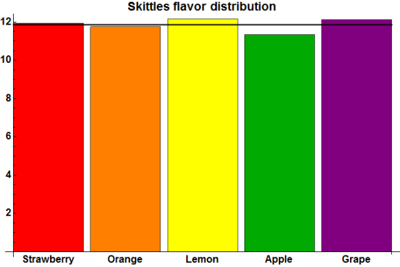
Average number of Skittles of each flavor in a pack. The assumed uniform average of 11.8547 Skittles of each color is shown by the black line.

Somewhat unfortunately, this data set potentially adds fuel to the frequent accusation that the yellow Skittles dominate. However, I leave it to an interested reader to consider and analyze whether this departure from uniformity is significant.

How accurate was our prior assumed distribution for the total number of Skittles in each pack? The following figure shows the observed distribution from this sample of 468 packs, with the mean of 59.2735 Skittles per pack shown in red.

Histogram of total number of Skittles in each pack. The mean of 59.2735 is shown in red.

Although our prior assumed average of 60 Skittles per pack was reasonable, there is strong evidence against our assumption of independence from one pack to the next, as shown in the following figure. The x-axis indicates the pack number from 1 to 468, and the y-axis indicates the number of Skittles in the pack, either total (in black) or of each individual color. The vertical grid lines show the grouping of 36 packs per box.

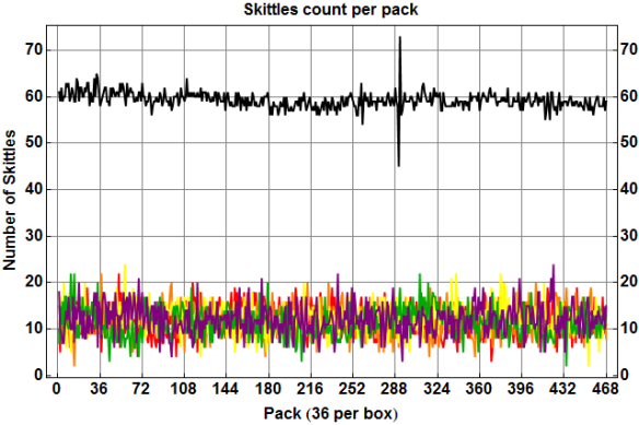
Number of Skittles per pack (total and of each color) vs. pack number.

The colored curves at bottom really just indicate the frequency and extent of outliers for the individual flavors; for example, we can see that every color appeared on at least 2 and at most 24 Skittles in every pack. The most interesting aspect of this figure, though, is the consecutive spikes in total number of Skittles shown by the black curve, with the minimum of 45 Skittles in pack #291 immediately followed by the maximum of 73 Skittles in pack #292. (See this past analysis of a single box of 36 packs that shows similar behavior.) This suggests that the dispenser that fills each pack targets an amortized rate of weight or perhaps volume, got jammed somehow resulting in an underfilled pack, and in getting “unjammed” overfilled the subsequent pack.

This is admittedly just speculation; note, for example, that the 36 packs in each box are relatively free to shift around, and I made only a modest effort to pull packs from each box in a consistent “top to bottom, front to back” order as I recorded them. So although each group of 36 packs in this data set definitely come from the same box, the order of packs within each group of 36 does not necessarily correspond to the order in which the packs were filled at the factory.

At any rate, if the objective of this experiment were to obtain a representative “truly random” sample of packs of Skittles, then the above behavior suggests that buying these 36-pack boxes in bulk is probably not recommended.

Stopping rule

Finally, one additional caveat: fortunately the primary objective of this experiment was not to obtain a “truly random” sample, but only to confirm the predicted “ease” with which we could find a pair of identical packs of Skittles. However, suppose that we did want to use this data set as a “truly random” sample… and further suppose that we could eliminate the practical imperfections suggested above, so that each pack was indeed a theoretically perfect, independent random sample.

Then even in this clean room thought experiment, we still have a problem: by stopping our sampling procedure upon encountering a duplicate, we have biased the distribution of possible resulting sample data sets! This can perhaps be most clearly seen with a simpler setup that allows an analytical solution: suppose that each pack contains just Skittles, and each individual Skittle is independently equally likely to be one of just possible colors, red or green. If we collect any fixed number of sample packs, then we should expect to observe an “all-red” pack with two red Skittles exactly 1/4 of the time. But if we instead collect sample packs until we observe a first duplicate, and then count the fraction that are all red, the expected value of this fraction is slightly less than 1/4 (181/768, to be exact). That is, by stopping with a duplicate, we are less likely to even get a chance to observe the more rare all-red (or all-green) packs.

It’s an interesting problem to quantify the extent of this effect (which I suspect is vanishingly small) with actual packs of Skittles, where the numbers of candies are larger, and the probabilities of those “extreme” compositions such as all reds is so small as to be effectively zero.