What are Ford circles?

Posted on November 18, 2025 by kjytay

The Ford circles, introduced by L. R. Ford in his 1938 paper (Reference 1), are a family of circles that are all tangent to the $x$ -axis at rational points. For each rational number $p/q$ with $\text{gcd}(p,q) = 1$ , the Ford circle $C[p,q]$ is defined as the circle centered at $\left( \dfrac{p}{q}, \dfrac{1}{2q^2} \right)$ with radius $\dfrac{1}{2q^2}$ .

Plotting these circles reveals how special they are:

A plot of Ford circles. Figure 2 from Reference 1.

No two of the circles intersect at each other at two distinct points. More interestingly, we can characterize which circles are tangent to each other!

Theorem (Section 1 of Ford (1938)). Two Ford circles $C[p,q]$ and $C[P,Q]$ are tangent to each other if and only if $|Pq - pQ| = 1$ .

The Ford circles are related to many different ideas in mathematics; I’ll just mention some of the properties I found interesting.

Theorem (Theorem 3 & 4 of Ford (1938)). If $C[P,Q]$ is tangent to $C[p,q]$ , then all the circles tangent to $C[p,q]$ are $C[P+np, Q+nq]$ , where $n$ takes on all integral values. In particular, across all possible values of $(P_n, Q_n) = (P+np, Q+nq)$ , exactly two have denominators numerically smaller than $q$ , and these correspond to the two tangent circles that are larger than $C[p, q]$ .

Consider the inequality

$\begin{aligned} \left| \frac{p}{q} - \omega \right| < \frac{k}{q^2}. \qquad -(1) \end{aligned}$

Dirichlet showed that:

If $\omega$ is irrational, then the inequality is satisfied by infinitely many fractions $p/q$ for $k = 1$ , and
If $\omega$ is rational, then the inequality is satisfied by only finitely many fractions, no matter how large $k$ is.

Ford used Ford circles to improve the result for irrational $\omega$ :

Theorem (Theorem 5 of Ford (1938)). If $k = 1/\sqrt{5}$ , then for each irrational $\omega$ there are infinitely many fractions $p/q$ that satisfy $(1)$ . However, if $k < 1/\sqrt{5}$ , then there are irrationals $\omega$ such that $(1)$ holds for only finitely many fractions.

Ford circles are intimately connected with the Farey sequence: see References 1 & 3 for example.

The circle for the mediant touches the other two circles. (Taken from Reference 3.)

Finally, the sum of the areas of the Ford circles involves the Riemann zeta function $\zeta$ ! The result with a short proof is available in Wikipedia (Reference 2).

Theorem (Wikipedia). Let $A$ be the total area of the Ford circles $\left\{ C[p,q]: 0 < p/q \leq 1 \right\}$ . Then $A = \dfrac{45}{2}\dfrac{\zeta(3)}{\pi^3}$ .

References:

L. R. Ford (1938). Fractions.
Wikipedia. Ford circle.
ThatsMaths. Ford Circles & Farey Series.

Some stochastic calculus notes

Posted on August 22, 2025 by kjytay

We define the Itô integral as

$\begin{aligned} \int_0^t X_s dW_s &= \lim_{k \rightarrow \infty} \sum_{i=1}^k X_{t_{k, i-1}} (W_{t_{k,i}} - W_{t_{k,i-1}}), \end{aligned}$

where the partition $0 = t_{k,0} < t_{k,1} < \dots < t_{k,k} = t$ gets increasingly fine as $k \rightarrow \infty$ , and $\{ W_t \}$ is a standard Wiener process (Brownian motion).

The Itô integral is defined for stochastic processes $\{X_s\}$ that satisfy the following two assumptions (let’s call them the “Itô integral assumptions”):

The paths of $\{X_s\}$ do not “blow up”, i.e. $\int_0^t X_s^2 ds < \infty$ with probability 1 for every $t < \infty$ , and
$\{X_s\}$ is a non-anticipating process.

Theorem (Itô integral is zero on average). Suppose $\{X_s\}$ is such that its Itô integral exists, and in addition suppose that $\displaystyle\int_0^t \mathbb{E}[X_s^2] ds < \infty$ . Then

$\begin{aligned} \mathbb{E}\left[ \int_0^t X_s dW_s \right] = 0. \end{aligned}$

Theorem (Itô’s formula). Suppose that $f(t, x)$ is differentiable in $t$ and twice differentiable in $x$ . Assume that $\{ W_t \}$ is a standard Wiener process. Then

$\begin{aligned} f(t, W_t) &= f(0,0) + \int_0^t \dfrac{\partial f}{\partial t}(u, W_u)du + \int_0^t \dfrac{\partial f}{\partial x}(u, W_u)dW_u + \frac{1}{2}\int_0^t \dfrac{\partial^2 f}{\partial x^2} (u, W_u) du. \end{aligned}$

An Itô process is a stochastic process $\{ I_s \}$ of the form

$\begin{aligned} I_t = I_0 + \int_0^t X_s ds + \int_0^t Z_s dW_s, \end{aligned}$

where $\{ X_s\}$ and $\{ Z_s\}$ are non-anticipating processes satisfying the Itô integral assumptions and $I_0$ is a constant.

Theorem (Itô integral of Itô process is itself an Itô process). Let $\{ I_t \}$ be as above and let $\{ Y_t \}$ be a non-anticipating process. Then

$\begin{aligned} \int_0^t Y_s dI_s &= \lim_{k \rightarrow \infty} \sum_{i=1}^k Y_{t_{k, i-1}} (I_{t_{k,i}} - I_{t_{k,i-1}}) \end{aligned}$

exists and is equal to

$\begin{aligned} \int_0^t Y_s dI_s &= \int_0^t Y_s X_s ds + \int_0^t Y_s Z_s dW_s, \end{aligned}$

provided $\{ Y_s X_s \}$ and $\{ Y_s Z_s \}$ satisfy the appropriate properties so the integrals exist.

Theorem (Itô’s formula for Itô processes). Let $\{ I_t \}$ be an Itô process of the form

$\begin{aligned} I_t = I_0 + \int_0^t X_s ds + \int_0^t Z_s dW_s, \end{aligned}$

and let $f(t, x)$ be differentiable in $t$ and twice differentiable in $x$ . Then

$\begin{aligned} f(t, I_t) &= f(0,I_0) + \int_0^t \dfrac{\partial f}{\partial t}(u, I_u)du + \int_0^t \dfrac{\partial f}{\partial x}(u, I_u)dI_u + \frac{1}{2}\int_0^t \dfrac{\partial^2 f}{\partial x^2} (u, I_u) Z_u^2 du. \end{aligned}$

Theorem (Itô isometry). Let $I_t = \displaystyle\int_0^t Z_s dW_s$ . Then

$\begin{aligned} \mathbb{E} \left[ \left( \int_0^t Z_s dW_s \right)^2 \right] = \mathbb{E} \left[ \int_0^t Z_s^2 ds \right]. \end{aligned}$

A probability puzzle involving random fractions

Posted on July 12, 2025 by kjytay

I came through this interesting probability brainteaser on Youtube today:

Let $X$ and $Y$ be independent random draws from the uniform distribution on $[0,1]$ .

a. Round the fraction $Y/X$ to the nearest integer. What is the probability that this integer is even?

b. Instead of rounding to the nearest integer, take the floor of the fraction $Y/X$ . What is the probability that this integer is even?

Stop scrolling if you’d like to give this problem a go, as the answer is below. Here is some R code performing a Monte Carlo simulation:

N <- 10000  # no. of simulations

set.seed(1)
X <- runif(N)
Y <- runif(N)
Z <- Y / X

# part (a)
sum(round(Z) %% 2 == 0) / N

# part (b)
sum(floor(Z) %% 2 == 0) / N

Interestingly, the answer to part (a) involves $\pi$ while the answer to part (b) involves $e$ ! More precisely, the answers are $\dfrac{5-\pi}{4}$ and $1 - \dfrac{\log 2}{2}$ (natural log).

The problem is actually not that difficult once we visualize all possible $(X, Y)$ pairs as points on the $[0,1] \times [0,1]$ square. Let’s solve (a) first. We want to find the areas of this square which correspond to $(X, Y)$ pairs such that $Y/X$ rounds to an even integer.

First, consider which $(X,Y)$ lead to $Y/X$ rounding to 0. They are the points such that

$\begin{aligned} Y/X < 1/2 \quad \Leftrightarrow \quad Y < \frac{1}{2}X. \end{aligned}$

This corresponds to the red triangle below (all pictures are screenshots from Reference 1), which has area 1/4:

Next, consider which $(X,Y)$ lead to $Y/X$ rounding to 2. They are the points such that

$\begin{aligned} 3/2 \leq Y/X < 5/2 \quad \Leftrightarrow \quad \frac{3}{2} X \leq Y < \frac{5}{2}X. \end{aligned}$

This refers to the area between the lines $Y = \frac{3}{2}X$ and $Y = \frac{5}{2}X$ , which corresponds to the second red triangle below:

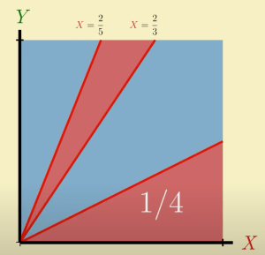
This triangle has height 1 and base length $\dfrac{2}{3} - \dfrac{2}{5}$ , and so has area $\dfrac{1}{2} \left( \dfrac{2}{3} - \dfrac{2}{5} \right)$ .

It’s not hard to generalize this to $Y/X$ which round to larger even integers:

The required probability is

$\begin{aligned} &\frac{1}{4} + \frac{1}{2} \left( \frac{2}{3} - \frac{2}{5} \right) + \frac{1}{2} \left( \frac{2}{7} - \frac{2}{9} \right) + \frac{1}{2} \left( \frac{2}{11} - \frac{2}{13} \right) + \dots \\ &\quad = \frac{1}{4} + 1 - 1 + \frac{1}{3} - \frac{1}{5} + \frac{1}{7} - \frac{1}{9} + \frac{1}{11} - \frac{1}{13} + \dots \\ &\quad = \frac{5}{4} - \left( 1 - \frac{1}{3} + \frac{1}{5} - \frac{1}{7} + \frac{1}{9} - \frac{1}{11} + \dots \right) \\ &\quad = \frac{5 - \pi}{4}, \end{aligned}$

where the last line is due to Leibniz’s formula for $\pi$ .

We can use this same approach for (b). For the first 2 triangles,

$\begin{aligned} Y/X < 1 \quad &\Leftrightarrow \quad Y < X, \\ 2 \leq Y/X < 3 \quad &\Leftrightarrow \quad 2X \leq Y < 3X, \end{aligned}$

which correspond to the two red triangles below:

Generalizing to larger integers:

The required probability is

$\begin{aligned} &\frac{1}{2} + \frac{1}{2} \left( \frac{1}{2} - \frac{1}{3} \right) + \frac{1}{2} \left( \frac{1}{4} - \frac{1}{5} \right) + \frac{1}{2} \left( \frac{1}{6} - \frac{1}{14} \right) + \dots \\ &\quad = \frac{1}{2} \left( 1 + \frac{1}{2} - \frac{1}{3} + \frac{1}{4} - \frac{1}{5} + \dots \right) \\ &\quad = 1 - \frac{1}{2} \left( 1 - \frac{1}{2} + \frac{1}{3} - \frac{1}{4} + \dots \right). \end{aligned}$

The infinite sum in the parentheses is known as the alternating harmonic series and is equal to $\log 2$ (several proofs, one here), and so the desired probability is $1 - \frac{1}{2}\log 2$ .

References:

Morphocular (2025). “The answer involves π because why wouldn’t it? 🙃”

The Leibniz integral rule

Posted on April 2, 2025 by kjytay

The Leibniz integral rule for differentiation under the integral sign is super important but I keep forgetting it. Am writing this post as a convenient bookmark for myself.

Let $f(x,t)$ be a function such that both $f(x,t)$ and its partial derivative $f_x(x,t)$ are continuous in $t$ and $x$ in some region of the $xt$ -plane, including $a(x) \leq t \leq b(x)$ , $x_0 \leq x \leq x_1$ . Also suppose that the functions $a(x)$ and $b(x)$ are both continuous and both have continuous derivatives for $x_0 \leq x \leq x_1$ . Then, for $x_0 \leq x \leq x_1$ ,

$\begin{aligned} \frac{d}{dx} \left( \int_{a(x)}^{b(x)} f(x,t)dt \right) &= f(x, b(x)) \cdot \frac{d}{dx}b(x) - f(x, a(x)) \cdot \frac{d}{dx}a(x) \\ &\qquad + \int_{a(x)}^{b(x)} \frac{\partial}{\partial x} f(x, t)dt. \end{aligned}$

In the special case where $a(x) = a$ and $b(x) = b$ are constants, we have

$\begin{aligned} \frac{d}{dx} \left( \int_a^b f(x,t)dt \right) &= \int_a^b \frac{\partial}{\partial x} f(x, t)dt. \end{aligned}$

The maximum number of equidistant points in R^n is…

Posted on April 2, 2025 by kjytay

Assume that we are in $n$ -dimensional Euclidean space $\mathbb{R}^n$ . What is the maximum number of points $x_1, x_2, \dots \in \mathbb{R}^n$ you can have such that they are equidistant, i.e. $\| x_i - x_j \|_2 = D$ for all $i \neq j$ , where $D$ is some fixed constant?

The answer is $n + 1$ . Turns out it was pretty difficult to find a reference that proved this in an easy-to-understand presentation (for me), so I’m writing my own version (largely based on Reference 1).

We prove that the maximum number of equidistant points in $\mathbb{R}^n$ is $n+1$ in two parts:

There exists a set of $n + 1$ equidistant points in $\mathbb{R}^n$ .
There cannot be more than $n+1$ equidistant points in $\mathbb{R}^n$ .

There exists a set of $n + 1$ equidistant points in $\mathbb{R}^n$

We prove existence by explicitly constructing such a set. For $i = 1, \dots, n$ , let $x_i$ be the vector with all zeros except for a 1 in the $i$ th position. For any $i \neq j$ , it is easy to see that

$\begin{aligned} \| x_i - x_j \|_2^2 = 1^2 + 1^2 = 2. \end{aligned}$

Define $x_{n+1} = \begin{pmatrix} -t & -t & \dots & -t \end{pmatrix}^\top$ , where $t$ is to be defined later. For any $i = 1, \dots, n$ , we have

$\begin{aligned} \| x_{n+1} - x_i \|_2^2 &= (n-1)t^2 + (t+1)^2 \\ &= nt^2 + 2t + 1. \end{aligned}$

If we set $t = \dfrac{-1 + \sqrt{1 + n}}{n}$ , then

$\begin{aligned} \| x_{n+1} - x_i \|_2^2 &= \frac{(-1 + \sqrt{1 + n})^2}{n} + \frac{2(-1 + \sqrt{1 + n})}{n} + 1 \\ &= \frac{1 + (1+n) - 2\sqrt{1+n}}{n} + \frac{2\sqrt{1+n} - 2}{n} + 1 \\ &= 2, \end{aligned}$

meaning $x_1, \dots, x_{n+1}$ are all equidistant from each other.

There cannot be more than $n+1$ equidistant points in $\mathbb{R}^n$ .

To prove this statement, we first need to prove a key lemma:

Lemma. If $\{ x_1, \dots, x_m \}$ are all equidistant, then the set of differences $\{ x_1 - x_2, \dots, x_1 - x_m \}$ is a set of $m - 1$ linearly independent vectors.

Proof of lemma: The statement is trivially true for $m = 1$ and $m = 2$ . Assume that $m \geq 3$ . Assume we have coefficients $\alpha_j$ such that

$\begin{aligned} \mathbf{0} = \sum_{j \neq 1} \alpha_j (x_1 - x_j). \end{aligned}$

Take any $k \neq 1$ and take a dot product of both sides above with $(x_1 - x_k)$ :

$\begin{aligned} 0 &= \alpha_k \| x_1 - x_k \|_2^2 + \sum_{j \neq 1, k} \alpha_j (x_1 - x_j) \cdot (x_1 - x_k). \qquad -(1) \end{aligned}$

Since

$\begin{aligned} D^2 &= \| x_j - x_k \|_2^2 = \| (x_1 - x_k) - (x_1 - x_j) \|_2^2 \\ &= \| x_1 - x_k \|_2^2 + \| x_1 - x_j \|_2^2 - 2 (x_1 - x_j) \cdot (x_1 - x_k), \\ (x_1 - x_j) \cdot (x_1 - x_k) &= D^2 / 2, \end{aligned}$

we can plug this into $(1)$ to get

$\begin{aligned} 0 &= 2 \alpha_k D^2 + D^2 \sum_{j \neq 1, k} \alpha_j, \\ 0 &= \alpha_k + \sum_{j \neq 1} \alpha_j. \qquad -(2) \end{aligned}$

Since $(2)$ applies for any $k \neq 1$ , for any $k \neq 1$ and $k' \neq 1$ with $k \neq k'$ , we must have

$\begin{aligned} \alpha_k + \sum_{j \neq 1} \alpha_j &= 0 = \alpha_{k'} + \sum_{j \neq 1} \alpha_j, \\ \alpha_k &= \alpha_{k'}, \end{aligned}$

i.e. all the $\alpha_2, \alpha_3, \dots$ are equal. But plugging this back into $(2)$ shows that all of them must be zero, implying that $\{ x_1 - x_2, \dots, x_1 - x_m \}$ are linearly independent. This proves the lemma.

Now let’s use the lemma to prove our statement that there cannot be more than $n+1$ equidistant points in $\mathbb{R}^n$ . Let $\{ x_1, \dots, x_m \}$ be the largest possible set of equidistant points in $\mathbb{R}^n$ . The lemma tells us that we can find a linearly independent set of vectors of size $m - 1$ . Since there are at most $n$ linearly independent vectors in $\mathbb{R}^n$ , we must have $m -1 \leq n$ , or $m \leq n+1$ .

References:

StackExchange. Proof maximum number of equidistant points for a given dimension [duplicate].
StackExchange. n points can be equidistant from each other only in dimensions ≥n−1?

What is the Buenos Aires constant?

Posted on February 20, 2025 by kjytay

I learned about the Buenos Aires constant from John Cook’s blog post. (If you haven’t realized already, I draw a lot of inspiration from his blog! It’s a great read and I highly recommend subscribing to it.)

The Buenos Aires constant, proposed by Fridman et al. (Reference 1) is

$\lambda = 2.92005097731613\dots$

and has an interesting property:

Proposition 1. Let $f_1 = \lambda$ be as above, and define the sequences

$\begin{aligned} g_n &= \left\lfloor f_n \right\rfloor, \\ f_{n+1} &= g_n (f_n - g_n + 1). \end{aligned}$

Then $g_1, g_2, \dots$ generates the complete sequence of primes $2, 3, 5, 7, \dots$ .

That seems really amazing! It becomes a little less amazing when you realize that $\lambda$ is defined as an infinite sum involving all the primes themselves… if $p_n$ denotes the $n$ th prime (starting with $p_1 = 2$ ), the Buenos Aires constant is defined as

$\begin{aligned} \lambda &= \sum_{k=1}^\infty \dfrac{p_k - 1}{\prod_{i=1}^{k-1} p_i} \\ &= \frac{2-1}{1} + \frac{3 - 1}{2} + \frac{5 - 1}{2 \cdot 3} + \dots \end{aligned}$

The proof, also in Reference 1, is short (about a page long) and relies solely on Bertrand’s postulate, i.e. the primes satisfy the inequalities $p_{n-1} < p_n < 2p_{n-1} - 1$ for all $n$ . In the paper, they actually prove this next proposition, and obtain Proposition 1 as a corollary:

Proposition 2. Let $p_1, p_2, \dots$ be a sequence of positive integers satisfying $p_{n-1} < p_n < 2p_{n-1} - 1$ for all $n$ (take $p_0 = 1$ ). Define the sequences

$\begin{aligned} f_1 &= \sum_{k=1}^\infty \dfrac{p_k - 1}{\prod_{i=1}^{k-1} p_i}, \\ g_n &= \left\lfloor f_n \right\rfloor, \\ f_{n+1} &= g_n (f_n - g_n + 1). \end{aligned}$

Then $g_n = p_n$ for all $n$ .

Why is it called the Buenos Aires constant? From the paper:

Dylan, Juli, Bruno and Massi are a group of 18/19-year-old friends from Buenos Aires, Argentina. The original idea came to Juli while having a shower. Bruno calculated the prime-generating constant, first by brute-force and then by finding its formula. As the investigation continued, Juli and Bruno were joined by Massi and Dylan. Later, the team contacted mathematician James Grime who helped by tidying up some of the proofs and writing this note. So ∞ thanks to James!

And that’s how fun math is done!

References:

Fridman, D., et al. (2019). A Prime-Representing Constant.

A theorem on interpolation error bound

Posted on September 11, 2024 by kjytay

I recently came across this theorem on John Cook’s blog that I wanted to keep for myself for future reference:

Theorem. Let $f$ be a function so that $f^{(n+1)}$ is continuous on $[a,b]$ and satisfies $|f^{(n+1)}(x)| \leq M$ . Let $p$ be a polynomial of degree $\leq n$ that interpolates $f$ at $n + 1$ equally spaced nodes in $[a,b]$ , including the end points. Then on $[a,b]$ ,

$\begin{aligned} |f(x) - p(x)| \leq \dfrac{1}{4(n+1)} M \left( \dfrac{b-a}{n} \right)^{n+1}. \end{aligned}$

A worked example

Let’s see what this looks like for a simple worked example. Consider the function $f(x) = \sin x$ on the interval $[0, \pi]$ , and let $n = 2$ , which means we are looking at a quadratic approximation.

The third derivative of $f$ is $f^{(3)}(x) = -\cos x$ , so we can set $M = 1$ . The interpolating quadratic function needs to go through $(0, 0)$ , $(\pi/2, 1)$ and $(\pi, 0)$ , which by Lagrange’s interpolating formula, is

$\begin{aligned} p(x) = \dfrac{(x-\pi/2)(x-\pi)}{(0-\pi/2)(0-\pi)} \cdot 1. \end{aligned}$

According to the theorem, on $[0, \pi]$ we have

$\begin{aligned} |f(x) - p(x)| \leq \dfrac{1}{4(2+1)} (1) \left( \dfrac{\pi-0}{2} \right)^{2+1} = \dfrac{\pi^3}{96} \approx 0.32. \end{aligned}$

The left plot below shows $f$ and its quadratic approximation, the right plots shows $f(x) - p(x)$ . As you can see from the y-axis on the right plot, the bound is pretty loose for this example.

We can run through the example with $n = 3$ as well (cubic approximation). The 4th derivative of $f$ is $f^{(4)}(x) = \sin x$ , so we can set $M = 1$ . The interpolating cubic function needs to go through $(0, 0)$ , $(\pi/3, \sqrt{3}/2)$ , $(2\pi/3, \sqrt{3}/2)$ and $(\pi, 0)$ . We can use Lagrange’s interpolating formula again, though the formula is much messier this time.

According to the theorem, on $[0, \pi]$ we have

$\begin{aligned} |f(x) - p(x)| \leq \dfrac{1}{4(3+1)} (1) \left( \dfrac{\pi-0}{3} \right)^{3+1} = \dfrac{\pi^4}{1296} \approx 0.075. \end{aligned}$

Below are the analogous plots for the cubic approximation. Again the theorem is true but the bound is not as loose as before.

Here are both the quadratic and cubic approximations on the same plot:

Code to reproduce the plots can be found here.

What is Craig’s formula for the Gaussian Q-function?

Posted on September 5, 2024 by kjytay

I recently learned of Craig’s formula for the Gaussian Q-function from this blog post from John Cook. Here is the formula:

Proposition (Craig’s formula). Let $Z$ be a standard normal random variable. Then for any $z \geq 0$ , defining

$\begin{aligned} \mathbb{P}\{ Z \geq z\} = Q(z) = \dfrac{1}{\sqrt{2\pi}} \int_z^\infty \exp \left( - \dfrac{u^2}{2} \right) du, \end{aligned}$

we have

$\begin{aligned} \dfrac{1}{\sqrt{2\pi}} \int_z^\infty \exp \left( - \dfrac{u^2}{2} \right) du = \dfrac{1}{\pi} \int_0^{\pi / 2} \exp \left( -\dfrac{z^2}{2 \sin^2 \theta} \right) d\theta . \end{aligned}$

This formula was first presented in Craig 1991 (Reference 1). John Cook notes that Craig’s formula is a better integral representation for $Q(z)$ from the perspective of numerical integration.

I tried proving this identity on my own without success. After some googling, I found a paper (Stewart 2017, Reference 2) that outlines 5 different proofs of the formula! The paper also notes that

“Currently no simple substitution which takes the Q-function from its canonical form to the form given by (6) is known,”

which made me feel a little better about my math skills. None of the proofs are particularly short, so instead of reproducing here, I’ll just provide the titles for each method to give a sense of what was involved:

Conversion to polar coordinates
Using an auxiliary function
Solution of a differential equation
Differentiating under the integral sign (again)
Another change of variables

Reference 2 also notes that there is a cosine form for Craig’s formula (the $\sin$ in the original formula is replaced with a $\cos$ ):

$\begin{aligned} Q(z) = \dfrac{1}{\pi} \int_0^{\pi / 2} \exp \left( -\dfrac{z^2}{2 \cos^2 \theta} \right) d\theta .\end{aligned}$

Finally, Beaulieu 2013 (Reference 3) presents an analogous formula for the square of the Q-function (the only change on the RHS is in the limits of integration):

$\begin{aligned} Q^2(z) = \dfrac{1}{\pi} \int_0^{\pi / 4} \exp \left( -\dfrac{z^2}{2 \sin^2 \theta} \right) d\theta, \end{aligned}$

and notes that it is a special case of a more general formula which is proved in the paper:

$\begin{aligned} Q(x)Q(y) = \dfrac{1}{2\pi} \int_0^{\theta_0} \exp \left( -\dfrac{y^2}{2 \sin^2 \theta} \right) d\theta + \dfrac{1}{2\pi} \int_{\theta_0}^{\pi / 2} \exp \left( -\dfrac{x^2}{2 \cos^2 \theta} \right) d\theta, \end{aligned}$

where $\theta_0 = \arctan (y/x)$ .

References:

Craig, J. W. (1991). A new, simple and exact result for calculating the probability of error for two-dimensional signal constellations.
Stewart, S. M. (2017). Some alternative derivations of Craig’s formula.
Beaulieu, N. C. (2013). Generalization of Craig’s Second Formula.

Paint roller puzzle in R

Posted on May 5, 2024 by kjytay

I recently learned of a simple logic puzzle from my daughter’s mathletes class (run by Coach K’s Mathletes) that I thought would be fun to code up. The puzzle is called “Paint Roller”, and is succinctly described in the image below:

If I were to relabel the rows as A, B and C and the columns as 1, 2 and 3, the image below shows how the correct solution paints the board step by step:

This is relatively simple to code up in R. The full code can be found at this link. The main function is play_game() which starts an interactive version of the game:

set.seed(1)
play_game(row_count = 4, col_count = 4)

This prints an image showing the start and end of the roller puzzle, and a prompt appears in the console asking you for the sequence that generated the end image.

The console will keep prompting you for sequences until you get the correct answer. The code also does some basic validation (e.g. check that the sequence contains valid characters and that no characters are duplicated).

If you get the correct answer, the image tells you that you won and the game ends. You can also enter Q at any time to end the game. When the game ends, it tells you the sequence it used to generate the board. Note that there can be more than one correct sequence: for example, ABC123 and CBA321 will produce the same board.

The play_game() function allows you to specify the number of rows and columns, as well as a custom color palette if you’d like:

set.seed(1)
play_game(row_count = 3, col_count = 4,
          color_list = c("green", "cyan", "magenta", "red", "orange", "yellow", "black"))

There are two other functions that might be of interest. The first is make_image(), which makes an image of the board for a given sequence:

make_image("AC1", row_count = 4, col_count = 3)

The other function is show_entire_sequence(), which shows how a sequence paints the board step-by-step. This is especially useful for helping kids visualize what is going on.

show_entire_sequence("A3BC21", row_count = 4, col_count = 4)

Both make_image() and show_entire_sequence() also have the optional color_list argument for setting custom color palettes.

How to prove Maclaurin’s inequality and Newton’s inequality

Posted on January 7, 2024 by kjytay

In this previous post, I used Maclaurin’s inequality to prove Sierpiński’s inequality. In this post, I show how Newton’s inequality can be used to prove Maclaurin’s inequality, and give a sketch of a proof of Newton’s inequality.

Statement of the theorems

Let $x_1, \dots, x_n$ be $n$ positive real numbers.For any integer $k \in \{ 1, \dots, n\}$ , define the symmetric sum and symmetric mean by

$\begin{aligned} S_k &= \sum_{1 \leq i_1 < \dots < i_k \leq n} x_{i_1} x_{i_2} \dots x_{i_k}, \\ M_k &= \dfrac{1}{\binom{n}{k}} S_k. \end{aligned}$

Note that this is different notation from my previous post. Here I am using $S$ for “sum” and $M$ for “mean”. For $k = 0$ , define $S_0 = M_0 = 1$ .

Theorem (Maclaurin’s inequality). $\begin{aligned} M_1 \geq M_2^{1/2} \geq \dots \geq M_n^{1/n}, \end{aligned}$

with equality when all the $x_i$ are equal.

Theorem (Newton’s inequality). For any $k \in \{ 1, \dots, n-1 \}$ ,

$\begin{aligned} M_k^2 \geq M_{k-1}M_{k+1}, \end{aligned}$

with equality when all the $x_i$ are equal.

Using Newton’s to prove Maclaurin’s

Using Newton’s inequality for $j = 1, \dots, k$ ,

$\begin{aligned} \prod_{j=1}^k M_j^{2j} &\geq \prod_{j=1}^k (M_{j-1}M_{j+1})^j \\ &= \prod_{j=0}^{k-1} M_j^{j+1} \prod_{j=2}^{k+1} M_j^{j-1} \\ &= M_0 \cdot M_1^2 \cdot M_k^{k-1} \cdot M_{k+1}^k \cdot \prod_{j=2}^{k-1} M_j^{2j}, \\ M_1^2 M_k^{2k} &\geq M_1^2 \cdot M_k^{k-1} \cdot M_{k+1}^k, \\ M_k^{k+1} &\geq M_{k+1}^k, \\ M_k^{1/k} &\geq M_{k+1}^{1/(k+1)}, \end{aligned}$

as desired.

Sketch proof of Newton’s inequality

There are several ways to prove Newton’s inequality (for e.g., see References 1 and 2). I think the most straightforward proof is by induction and with some algebraic manipulation. I sketch the approach here; full details can be found in Reference 1.

We prove Newton’s inequality via induction on $n$ . For $n = 2$ , the only possible value of $k$ is 1, and the inequality to be proven is $M_1^2 \geq M_2 M_0$ , which is simply the AM-GM inequality.

Now, assume that the inequality is true for some $n = m-1$ . We need to show that it is also true for $n = m$ . Fix the value of $k$ . Let $M_k$ ( $S_k$ resp.) denote the symmetric mean (sum resp.) for $x_1, \dots, x_m$ and let $M_k'$ ( $S_k'$ resp.) denote the symmetric mean (sum resp.) for $x_1, \dots, x_{m-1}$ . Then, by considering whether $x_m$ is in the term or not,

$\begin{aligned} S_k &= \sum_{1 \leq i_1 < \dots < i_k \leq m} x_{i_1} x_{i_2} \dots x_{i_k} \\ &= \sum_{1 \leq i_1 < \dots < i_k \leq m-1} x_{i_1} x_{i_2} \dots x_{i_k} + x_m \sum_{1 \leq i_1 < \dots < i_{k-1} \leq m-1} x_{i_1} x_{i_2} \dots x_{i_{k-1}} \\ &= S_k' + x_m S_{k-1}', \\ M_k &= \dfrac{1}{\binom{m}{k}} \left[ \binom{m-1}{k} M_k' + \binom{m-1}{k-1} x_m M_{k-1}' \right] \\ &= \dfrac{m-k}{m} M_k' + \dfrac{k}{m} x_m M_{k-1}'. \end{aligned}$

We need to show that $M_k^2 \geq M_{k-1}M_{k+1}$ . To do that, apply the identity above to each term of $M_{k-1}M_{k+1}$ , then apply the induction assumption and do some algebraic manipulation to get it to be $\leq M_k^2$ . (Details in Reference 1.)

References:

AoPS Online. Newton’s Inequality.
Cut The Knot. Newton’s and Maclaurin’s Inequalities.