In November 6th – 11th we had a face-to-face training course on “Meteorological Satellite Products and Applications for Mid-Latitudes” in Montevideo, Uruguay, organized by @AEMET_Esp / @AECID_es and @eumetsat, with participants from Argentina, Brazil, Chile, Mexico, Paraguay and Uruguay.
A great experience! The instructors covered different products and application areas: nowcasting, fog, ocean, fires, aerosol, vegetation, data access and processing, the new generation of satellites and more. And we also visited INUMET, the Uruguayan Institute of Meteorology.
The instructors were from Spain (AEMET), Portugal (EUMETSAT), Brazil (INPE) and Uruguay (FAU).
Many hands-on activities included! Participants presented their case studies / exercises using satellite data from @eumetsat / @LSA_SAF and @NOAASatellites, including Metop, Meteosat, GOES-East, GOES-West and NWP data from @ECMWF, using Python to create their images! @PyTrollOrg
GLM FED, TOE and MFA + ABI Band 13 (10.3 μm) – Cylindrical Equidistant projection
After the preliminary tests and adjustments, the last thing we wanted to test was plotting the GLM FED, TOE and MFA gridded products in the cylindrical equidistant projection (so it can be overlayed with other products).
And that was possible thanks to the reprojection examples found on the excelent GOES package created by Joao Huamán (SENAMHI, Peru), that uses the pyproj and pyresample packages to do the task.
The GitHub repository has been updated with a third example:
GLM FED, TOE and MFA – Processed with Python using glmtools
After the preliminary tests, I’ve noticed some big differences between our plots and the plots available in the reference quick guides.
Thanks to Joseph Patton, research scientist from CISESS, ESSIC, University of Maryland-College Park, we were able to adjust the color scales and ranges and now the FED, TOA and MFA plots are very similar to the ones available in reference material.
Also, Joseph suggested a nice reference page: the College of DuPage website, that lets users overlay the GLM gridded products with their standard color bars on top of other satellite imagery in real-time. That would allow us to save some high-quality animations of GLM imagery to compare to our own output using glmtools. Great!
He also shared a presentation he gave for an AMS Short Course in March 2021 about the FED, MFA, and TOE gridded products and how to apply them in a few meteorological applications:
We would like to share with you the Applied Remote Sensing Training (ARSET) Program Online Resource Guide: 2015-2022 shared by Brock Blevins (NASA/ARSET Program):
It has a wide range of online resources addressing utilization of satellite data and products for various application areas (Climate & Resilience, Disasters, Health & Air Quality, Ecological Conservation, Water Resources, Capacity Building) freely available for everyone. Each online resource listed in the Guide is linked to a dedicated web page which has the recordings of the training sessions, presentation slides, as well as Q&A transcripts.
Some training resources are provided not only in English, but also in Spanish (it has “Bilingual” in its description).
We hope you find them useful!
Thanks Brock Blevins for sharing this information!
Developed by our colleagues from INPE, TATHU (Tracking and Analysis of Thunderstorms) is a Python package for tracking and analyzing the life cycle of Convective Systems (CS).
The package provides a modular and extensible structure, supports different types of geospatial data and proposes the use of Geoinformatics techniques and spatial databases in order to aid in the analysis and computational representation of the CS.
In addition, the package presents a conceptual model for defining the problem using abstract interfaces.
Note: The Portuguese word for “armadillo” is tatu which is derived from the Tupi language.
True Color RGB Composite overlayed with the NHC Tracking and Forecast – MARN El SalvadorGOES-16 Rainfall Rate / QPE product overlayed with the NHC Tracking and Forecast – MARN El SalvadorMARN El Salvador – SHOWCast Interface
Thanks for sharing William!
This Blog series shows the products developed by the community in the Americas. Most of them refers to data received from GNC-A, however, we also post the development with data received from other means. Please find below the other posts from this series:
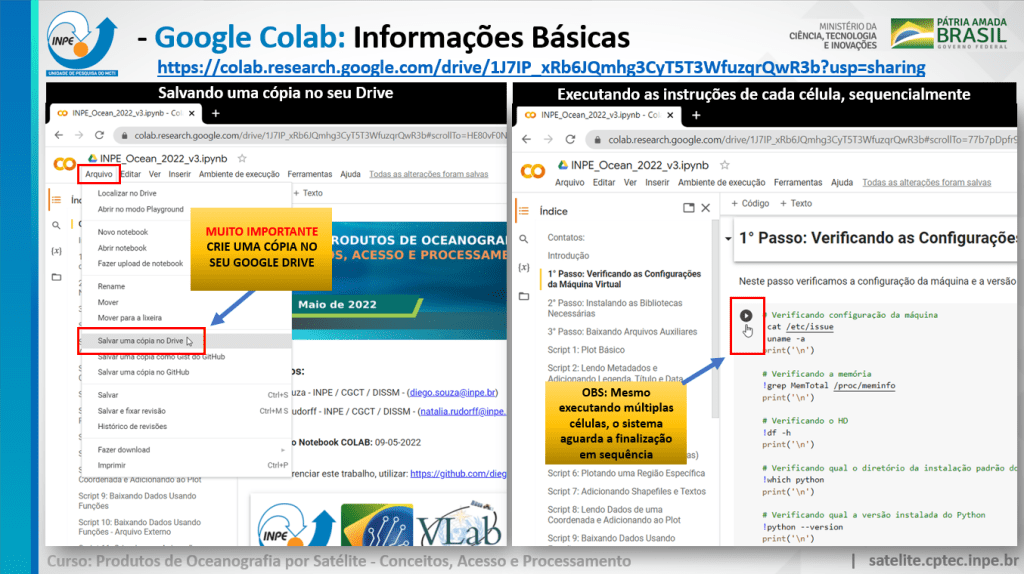
Prezados participantes do curso: “Produtos de Oceanogradia por Satélite – Conceitos, Acesso e Processamento”, segue abaixo o link do “notebook” interativo do Google Colab com as atividades do curso.
Este “notebook” interativo contém instruções para a instalação das ferramentas necessárias para a criação de scripts Python e a manipulação dos dados mostrados no curso. Todas as instruções e scripts são executados na nuvem, não sendo necessário instalar as ferramentas e baixar arquivos localmente, como no procedimento pré-curso. Para executar as instruções, clicar no ícone “Play” entre colchetes à esquerda de cada célula.
Para ter uma melhor experiência com a ferramenta e poder editar / salvar seus scripts, é imprescindível a criação de uma cópia no seu próprio Google Drive, em “Arquivo” -> “Salvar uma cópia no Drive”.
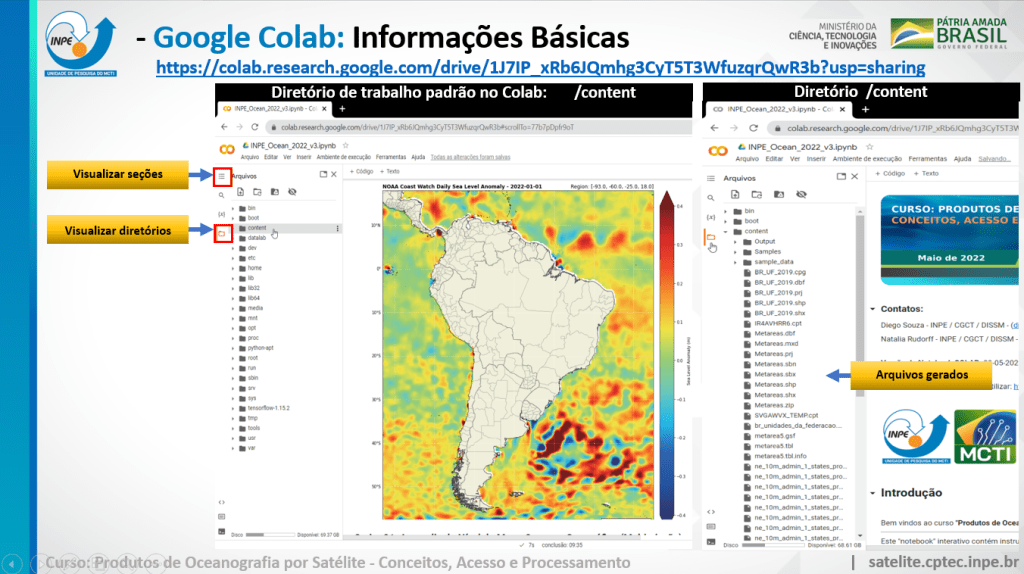
Seguem algumas orientações nas imagens abaixo (clique nas imagens para ampliar):
Criando uma cópia do “notebook” e executando as células sequencialmenteAdicionando células de código e de textoSeções, células de texto, células de código e sua saídaImpando as saídas das células de código, resetando o kernel Python e resetando a máquinaVisualizando seções e diretórios da máquina virtual
A test 2D array converted to GeoTIFF and opened in QGIS
We received the following question:
How can I generate a GeoTIFF from GOES-16 products?
The example code below demonstrates how to generate a GeoTIFF from a numpy array. This array could be your GOES-16 data or data from other satellites.
In this example, we’ll create a 2D array (30×30) with random numbers between 0 and 9:
# Create a test 2D array (randon numbers between 0 and 9)
import numpy as np
nlines = 30
ncolumns = 30
data = np.random.randint(0, 10, size=(nlines,ncolumns))
Then, we’ll export this array to GeoTIFF, for the region defined at the “extent” list:
#---------------------------------------------------------------------------------------------------------------------------
# Required modules
from osgeo import gdal, osr, ogr # Python bindings for GDAL
#---------------------------------------------------------------------------------------------------------------------------

def getGeoTransform(extent, nlines, ncols):
    resx = (extent[2] - extent[0]) / ncols
    resy = (extent[3] - extent[1]) / nlines
    return [extent[0], resx, 0, extent[3] , 0, -resy]

# Define the data extent (min. lon, min. lat, max. lon, max. lat)
extent = [-93.0, -60.00, -25.00, 18.00] # South America

# Export the test array to GeoTIFF ================================================

# Get GDAL driver GeoTiff
driver = gdal.GetDriverByName('GTiff')

# Get dimensions
nlines = data.shape[0]
ncols = data.shape[1]
nbands = len(data.shape)
data_type = gdal.GDT_Int16 # gdal.GDT_Float32

# Create a temp grid
#options = ['COMPRESS=JPEG', 'JPEG_QUALITY=80', 'TILED=YES']
grid_data = driver.Create('grid_data', ncols, nlines, 1, data_type)#, options)

# Write data for each bands
grid_data.GetRasterBand(1).WriteArray(data)

# Lat/Lon WSG84 Spatial Reference System
srs = osr.SpatialReference()
srs.ImportFromProj4('+proj=longlat +ellps=WGS84 +datum=WGS84 +no_defs')

# Setup projection and geo-transform
grid_data.SetProjection(srs.ExportToWkt())
grid_data.SetGeoTransform(getGeoTransform(extent, nlines, ncols))

# Save the file
file_name = 'my_test_data.tif'
print(f'Generated GeoTIFF: {file_name}')
driver.CreateCopy(file_name, grid_data, 0)

# Close the file
driver = None
grid_data = None

# Delete the temp grid
import os
os.remove('grid_data')
#==============================================================================
The code above generated a 2 KB GeoTIFF that could be opened in any GIS.
You may find a Google COLAB example in the following link: