# Training: Python and GOES-R Imagery: RGB Subplots
#---------------------------------------------------------------------------------------------
# Required modules
from netCDF4 import Dataset              # Read / Write NetCDF4 files
import matplotlib.pyplot as plt          # Plotting library
from datetime import datetime, timedelta # Library to convert julian day to dd-mm-yyyy
import cartopy, cartopy.crs as ccrs      # Plot maps
import numpy as np                       # Scientific computing with Python
#---------------------------------------------------------------------------------------------
#---------------------------------------------------------------------------------------------
# Open the GOES-R image
file1 = Dataset("OR_ABI-L2-CMIPF-M6C08_G16_s20191981200396_e20191981210104_c20191981210182.nc")
# Get the pixel values, and convert to Celsius
data1 = file1.variables['CMI'][:] - 273.15

# Open the GOES-R image
file2 = Dataset("OR_ABI-L2-CMIPF-M6C10_G16_s20191981200396_e20191981210116_c20191981210188.nc")
# Get the pixel values, and convert to Celsius
data2 = file2.variables['CMI'][:] - 273.15

# Open the GOES-R image
file3 = Dataset("OR_ABI-L2-CMIPF-M6C12_G16_s20191981200396_e20191981210111_c20191981210185.nc")
# Get the pixel values, and convert to Celsius
data3 = file3.variables['CMI'][:] - 273.15

# Open the GOES-R image
file4 = Dataset("OR_ABI-L2-CMIPF-M6C13_G16_s20191981200396_e20191981210116_c20191981210189.nc")
# Get the pixel values, and convert to Celsius
data4 = file4.variables['CMI'][:] - 273.15
#---------------------------------------------------------------------------------------------
#---------------------------------------------------------------------------------------------
# RGB Components
R = data1 - data2
G = data3 - data4
B = data1

# Minimuns, Maximuns and Gamma
Rmin = -26.2
Rmax = 0.6

Gmin = -43.2
Gmax = 6.7

Bmin = -29.25
Bmax = -64.65

# NOTE: FOR SOME REASON CAN'T PUT GREATER AND LESS THAN SIGNALS ON WORDPRESS
R[R[greater than]Rmax] = Rmax
R[R[less than]Rmin] = Rmin

G[G[greater than]Gmax] = Gmax
G[G[less than]Gmin] = Gmin

B[B[less than]Bmax] = Bmax
B[B[greater than]Bmin] = Bmin 

gamma_R = 1
gamma_G = 1
gamma_B = 1

# Normalize the data
R = ((R - Rmin) / (Rmax - Rmin)) ** (1/gamma_R)
G = ((G - Gmin) / (Gmax - Gmin)) ** (1/gamma_G)
B = ((B - Bmin) / (Bmax - Bmin)) ** (1/gamma_B) 

# Create the RGB
RGB = np.stack([R, G, B], axis=2)

# Eliminate values outside the globe
mask = (RGB == [R[0,0],G[0,0],B[0,0]]).all(axis=2)
RGB[mask] = np.nan
#---------------------------------------------------------------------------------------------
#---------------------------------------------------------------------------------------------
# Choose the plot size (width x height, in inches)
fig, (ax1, ax2, ax3) = plt.subplots(3,2, figsize=(9,7))
#---------------------------------------------------------------------------------------------
#---------------------------------------------------------------------------------------------
# Use the Geostationary projection in cartopy
ax1 = plt.subplot(121,projection=ccrs.Geostationary(central_longitude=-75.0, satellite_height=35786023.0))

# Geostationary extent
img_extent = (-5434894.67527,5434894.67527,-5434894.67527,5434894.67527)

# Eliminate values outside the globe
R[mask] = np.nan

# Plot the image
img1 = ax1.imshow(RGB, origin='upper', extent=img_extent)

# Add coastlines, borders and gridlines
ax1.coastlines(resolution='10m', color='white', linewidth=0.8)
ax1.add_feature(cartopy.feature.BORDERS, edgecolor='white', linewidth=0.5)
ax1.gridlines(color='white', alpha=0.5, linestyle='--', linewidth=0.5, xlocs=np.arange(-180, 180, 15), ylocs=np.arange(-180, 180, 15), draw_labels=False)

# Getting the ABI file date
add_seconds = int(file1.variables['time_bounds'][0])
date = datetime(2000,1,1,12) + timedelta(seconds=add_seconds)
date_format = date.strftime('%B %d %Y - %H:%M UTC')

# Add a title
ax1.set_title('GOES-16 Airmass RGB', fontweight='bold', fontsize=10, loc='left')
ax1.set_title('Full Disk \n' + date_format, fontsize=10, loc='right')
#---------------------------------------------------------------------------------------------
#---------------------------------------------------------------------------------------------
# Use the Geostationary projection in cartopy
ax2 = plt.subplot(322,projection=ccrs.Geostationary(central_longitude=-75.0, satellite_height=35786023.0))

# Geostationary extent
img_extent = (-5434894.67527,5434894.67527,-5434894.67527,5434894.67527)

# Eliminate values outside the globe
G[mask] = np.nan

# Plot the image
img2 = ax2.imshow(R, vmin=0, vmax=1, origin='upper', extent=img_extent, cmap='Reds')

# Add coastlines, borders and gridlines
ax2.coastlines(resolution='10m', color='black', linewidth=0.5)
ax2.add_feature(cartopy.feature.BORDERS, edgecolor='black', linewidth=0.5)
ax2.gridlines(color='black', alpha=0.5, linestyle='--', linewidth=0.5, xlocs=np.arange(-180, 180, 15), ylocs=np.arange(-180, 180, 15), draw_labels=False)

# Add a title
ax2.set_title('Red: 6.2 μm - 7.3 μm', fontweight='bold', fontsize=10, loc='center')
#---------------------------------------------------------------------------------------------
#---------------------------------------------------------------------------------------------
# Use the Geostationary projection in cartopy
ax3 = plt.subplot(324,projection=ccrs.Geostationary(central_longitude=-75.0, satellite_height=35786023.0))

# Geostationary extent
img_extent = (-5434894.67527,5434894.67527,-5434894.67527,5434894.67527)

# Plot the image
img3 = ax3.imshow(G, vmin=0, vmax=1, origin='upper', extent=img_extent, cmap='Greens')

# Add coastlines, borders and gridlines
ax3.coastlines(resolution='10m', color='black', linewidth=0.5)
ax3.add_feature(cartopy.feature.BORDERS, edgecolor='black', linewidth=0.5)
ax3.gridlines(color='black', alpha=0.5, linestyle='--', linewidth=0.5, xlocs=np.arange(-180, 180, 15), ylocs=np.arange(-180, 180, 15), draw_labels=False)

# Add a title
ax3.set_title('Green: 9.6 μm - 10.3 μm', fontweight='bold', fontsize=10, loc='center')
#---------------------------------------------------------------------------------------------
#---------------------------------------------------------------------------------------------
# Use the Geostationary projection in cartopy
ax4 = plt.subplot(326,projection=ccrs.Geostationary(central_longitude=-75.0, satellite_height=35786023.0))

# Geostationary extent
img_extent = (-5434894.67527,5434894.67527,-5434894.67527,5434894.67527)

# Eliminate values outside the globe
B[mask] = np.nan

# Plot the image
img4 = ax4.imshow(B, vmin=0, vmax=1, origin='upper', extent=img_extent, cmap='Blues')

# Add coastlines, borders and gridlines
ax4.coastlines(resolution='10m', color='black', linewidth=0.5)
ax4.add_feature(cartopy.feature.BORDERS, edgecolor='black', linewidth=0.5)
ax4.gridlines(color='black', alpha=0.5, linestyle='--', linewidth=0.5, xlocs=np.arange(-180, 180, 15), ylocs=np.arange(-180, 180, 15), draw_labels=False)

# Add a title
ax4.set_title('Blue: 6.2 μm (inverted)', fontweight='bold', fontsize=10, loc='center')
#---------------------------------------------------------------------------------------------
#---------------------------------------------------------------------------------------------
fig.subplots_adjust(wspace=.01,hspace=.01)
#---------------------------------------------------------------------------------------------
#---------------------------------------------------------------------------------------------
# Automatically adjust subplot parameters
fig.tight_layout()

# Save the image
plt.savefig('Image_13.png')

# Show the image
plt.show()

# Training: Python and GOES-R Imagery: GOES-16 and GOES-17 Subplots
#---------------------------------------------------------------------------------------------
# Required modules
from netCDF4 import Dataset              # Read / Write NetCDF4 files
import matplotlib.pyplot as plt          # Plotting library
from datetime import datetime, timedelta # Library to convert julian day to dd-mm-yyyy
import cartopy, cartopy.crs as ccrs      # Plot maps
import numpy as np                       # Scientific computing with Python
#---------------------------------------------------------------------------------------------
#---------------------------------------------------------------------------------------------
# Open the GOES-R image 1
file1 = Dataset("OR_ABI-L2-CMIPF-M6C13_G17_s20191981200341_e20191981209419_c20191981209474.nc")
# Get the pixel values
data1 = file1.variables['CMI'][:] - 273.15

# Open the GOES-R image 2
file2 = Dataset("OR_ABI-L2-CMIPF-M6C13_G16_s20191981200396_e20191981210116_c20191981210189.nc")
# Get the pixel values
data2 = file2.variables['CMI'][:] - 273.15
#---------------------------------------------------------------------------------------------
#---------------------------------------------------------------------------------------------
# Choose the plot size (width x height, in inches)
fig, (ax1, ax2) = plt.subplots(1,2, figsize=(12,7))
#---------------------------------------------------------------------------------------------
#---------------------------------------------------------------------------------------------
# Use the Geostationary projection in cartopy
ax1 = plt.subplot(121,projection=ccrs.Geostationary(central_longitude=-137.0, satellite_height=35786023.0))
# Geostationary extent
img_extent = (-5434894.67527,5434894.67527,-5434894.67527,5434894.67527)
# Plot the image
img1 = ax1.imshow(data1, vmin=-80, vmax=40, origin='upper', extent=img_extent, cmap='Greys')

# Add coastlines, borders and gridlines
ax1.coastlines(resolution='10m', color='white', linewidth=0.8)
ax1.add_feature(cartopy.feature.BORDERS, edgecolor='white', linewidth=0.5)
ax1.gridlines(color='white', alpha=0.5, linestyle='--', linewidth=0.5, xlocs=np.arange(-180, 180, 15), ylocs=np.arange(-180, 180, 15), draw_labels=False)
# Add a colorbar
fig.colorbar(img1, label='Brightness Temperature (°C)', extend='both', orientation='horizontal', pad=0.05, fraction=0.05)

# Getting the ABI file date
add_seconds = int(file1.variables['time_bounds'][0])
date = datetime(2000,1,1,12) + timedelta(seconds=add_seconds)
date_format = date.strftime('%B %d %Y - %H:%M UTC')

# Add a title
ax1.set_title('GOES-17 Band 13 (10.35 μm)', fontweight='bold', fontsize=10, loc='left')
ax1.set_title('Full Disk \n' + date_format, fontsize=10, loc='right')
#---------------------------------------------------------------------------------------------
# Use the Geostationary projection in cartopy
ax2 = plt.subplot(122,projection=ccrs.Geostationary(central_longitude=-75.0, satellite_height=35786023.0))

# Geostationary extent
img_extent = (-5434894.67527,5434894.67527,-5434894.67527,5434894.67527)

# Plot the image
img2 = ax2.imshow(data2, vmin=-80, vmax=40, origin='upper', extent=img_extent, cmap='Greys')

# Add coastlines, borders and gridlines
ax2.coastlines(resolution='10m', color='white', linewidth=0.8)
ax2.add_feature(cartopy.feature.BORDERS, edgecolor='white', linewidth=0.5)
ax2.gridlines(color='white', alpha=0.5, linestyle='--', linewidth=0.5, xlocs=np.arange(-180, 180, 15), ylocs=np.arange(-180, 180, 15), draw_labels=False)

# Add a colorbar
fig.colorbar(img2, label='Brightness Temperatures (°C)', extend='both', orientation='horizontal', pad=0.05, fraction=0.05)

# Getting the ABI file date
add_seconds = int(file2.variables['time_bounds'][0])
date = datetime(2000,1,1,12) + timedelta(seconds=add_seconds)
date_format = date.strftime('%B %d %Y - %H:%M UTC')

# Add a title
ax2.set_title('GOES-16 Band 13 (10.35 μm)', fontweight='bold', fontsize=10, loc='left')
ax2.set_title('Full Disk \n' + date_format, fontsize=10, loc='right')
#---------------------------------------------------------------------------------------------
#---------------------------------------------------------------------------------------------
fig.subplots_adjust(wspace=.02)
#---------------------------------------------------------------------------------------------
#---------------------------------------------------------------------------------------------
# Save the image
plt.savefig('Image_09.png')

# Show the image
plt.show()

# Training: Python and GOES-R Imagery: Script 8
#---------------------------------------------------------------------------------------------
# Required modules
from netCDF4 import Dataset              # Read / Write NetCDF4 files
import matplotlib.pyplot as plt          # Plotting library
from datetime import datetime, timedelta # Library to convert julian day to dd-mm-yyyy
import cartopy, cartopy.crs as ccrs      # Plot maps
import numpy as np                       # Scientific computing with Python
#---------------------------------------------------------------------------------------------
#---------------------------------------------------------------------------------------------
# Open the GOES-R image
file = Dataset("OR_ABI-L2-CMIPF-M6C13_G16_s20191981200396_e20191981210116_c20191981210189.nc")
# Get the pixel values
data = file.variables['CMI'][:] - 273.15
#---------------------------------------------------------------------------------------------
#---------------------------------------------------------------------------------------------
# Choose the plot size (width x height, in inches)
fig, (ax1, ax2) = plt.subplots(1,2, figsize=(12,7))
#---------------------------------------------------------------------------------------------
#---------------------------------------------------------------------------------------------
# Use the Geostationary projection in cartopy
ax1 = plt.subplot(121,projection=ccrs.Geostationary(central_longitude=-75.0, satellite_height=35786023.0))

# Geostationary extent
img_extent = (-5434894.67527,5434894.67527,-5434894.67527,5434894.67527)

# Plot the image
img1 = ax1.imshow(data, vmin=-80, vmax=40, origin='upper', extent=img_extent, cmap='Greys')

# Add coastlines, borders and gridlines
ax1.coastlines(resolution='10m', color='white', linewidth=0.8)
ax1.add_feature(cartopy.feature.BORDERS, edgecolor='white', linewidth=0.5)
ax1.gridlines(color='white', alpha=0.5, linestyle='--', linewidth=0.5, xlocs=np.arange(-180, 180, 15), ylocs=np.arange(-180, 180, 15), draw_labels=False)

# Add a colorbar
fig.colorbar(img1, label='Brightness Temperature (°C)', extend='both', orientation='horizontal', pad=0.05, fraction=0.05)

# Getting the ABI file date
add_seconds = int(file.variables['time_bounds'][0])
date = datetime(2000,1,1,12) + timedelta(seconds=add_seconds)
date_format = date.strftime('%B %d %Y - %H:%M UTC')

# Add a title
ax1.set_title('GOES-16 (GOES Imager Projection)\nBand 13 (10.35 μm)', fontweight='bold', fontsize=10, loc='left')
ax1.set_title('Full Disk \n' + date_format, fontsize=10, loc='right')

#---------------------------------------------------------------------------------------------
# Use the Geostationary projection in cartopy
ax2 = plt.subplot(122,projection=ccrs.PlateCarree(central_longitude=-75.0))

# Plot Extent
ax2.set_extent([-165.0, 15.0, -90.0, 90.0], crs=ccrs.PlateCarree())

# Add a background image
ax2.stock_img()

# Geostationary extent
img_extent = (-5434894.67527,5434894.67527,-5434894.67527,5434894.67527)

# Plot the image
img2 = ax2.imshow(data, vmin=-80, vmax=40, origin='upper', extent=img_extent, cmap='Greys', transform=ccrs.Geostationary(central_longitude=-75.0))

# Add coastlines, borders and gridlines
ax2.coastlines(resolution='10m', color='white', linewidth=0.8)
ax2.add_feature(cartopy.feature.BORDERS, edgecolor='white', linewidth=0.5)
ax2.gridlines(color='white', alpha=0.5, linestyle='--', linewidth=0.5, xlocs=np.arange(-180, 180, 15), ylocs=np.arange(-180, 180, 15), draw_labels=False)

# Add a colorbar
fig.colorbar(img2, label='Brightness Temperatures (°C)', extend='both', orientation='horizontal', pad=0.05, fraction=0.05)

# Add a title
ax2.set_title('GOES-16 (Cylindrical Projection)\nBand 13 (10.35 μm)', fontweight='bold', fontsize=10, loc='left')
ax2.set_title('Full Disk \n' + date_format, fontsize=10, loc='right')

fig.subplots_adjust(wspace=.02)
#---------------------------------------------------------------------------------------------
#---------------------------------------------------------------------------------------------
# Save the image
plt.savefig('Image_08.png')

# Show the image
plt.show()

 

Introducción al Procesamiento de Imagenes Satelitales con Python

Contacto: Si tiene alguna pregunta, comuníquese con:

Correo electrónico: [email protected]
Skype: diego.rsouza

Al final de los ejercícios, los participantes estarán capacitados a:

• Familiarizarse con algunas herramientas básicas para comenzar a manipular imágenes de satélite con Python
• Comprender cómo realizar operaciones básicas como:
  • Lectura de archivos NetCDF de GOES-R (GOES-16 o 17)
  • Hacer un plot básico de GOES-R y visualizar los valores de los píxeles (temperaturas de brillo / reflectancias)
  • Cambiar las escalas de colores, añadir un título y una barra de colores al plot
  • Agregar mapas de países, estados / provincias (y otros shapefiles)
  • Crear un plot de alta resolución
  • Crear una composición RGB

Duración: 1:20 h, incluyendo la instalación

Prerrequisitos:

Para este ejercicio, necesitaremos lo siguiente:

• Python 3.7 (nuestro lenguaje de programación)
• Un “Administrador de paquetes” (para instalar librerías)
• Un “Administrador de ‘Entornos Virtuales Python'” (para separar nuestros proyectos)
• Un editor de texto (para escribir nuestro código)
• Muestras de imágenes del GOES-R (los datos a manipular)

Para los primeros tres (“Python 3.7”, “Administrador de Paquetes” y “Administrador de ‘Entornos Virtuales Python'”), la herramienta “Miniconda” será suficiente.

En cuanto al editor de texto, hay muchas opciones disponibles (Spyder, PyCharm, Atom, Jupyter, etc.), pero por simplicidad, hoy usaremos “Notepad ++”.

Para las muestras de imágenes GOES-R, las descargaremos de la nube (Amazon). También puede obtenerlos de su estación GNC-A u otros mecanismos de recepción (GRB, etc.).

Pasos de la instalación:

1) Descargue e instale el Miniconda para Python 3.7 en el siguiente enlace (solo 60 MB):

Notas:

• Durante la instalación, no es necesario marcar “Add Anaconda to my Path environment variable“.
• Puede marcar “Register Anaconda as my default Python 3.7“
• La instalación tomará aproximadamente 5 minutos.

Crear un ‘Entorno Virtual de Python’ e instalar librerías:

2) Cree un entorno virtual Python llamado “workshop” e instale las siguientes bibliotecas y sus dependencias en este entorno:

• matplotlib: biblioteca para creación de plots
• netcdf4: leer / escribir archivos NetCDF
• cartopy: producir mapas y otros análisis de datos geoespaciales

Para hacerlo, abra el “Anaconda Prompt” recientemente instalado, como administrador:

E inserte el siguiente comando:

conda create --name workshop -c conda-forge matplotlib netcdf4 cartopy

Dónde:

workshop: el nombre de su entorno virtual Python. Podría ser cualquier cosa, como “satelite”, “goes”, etc.

matplotlib netcdf4 cartopy: las librerias que queremos instalar

Notas:

• Durante la instalación, escriba “y” + Enter para continuar, cuando se le solicite.
• Este procedimiento debería tomar aproximadamente 10 minutos.

Finalmente, active el entorno virtual Python recién creado con el siguiente comando:

activate workshop

Nota: Si está utilizando Linux, use el comando “source activate workshop“

Informaciones adicionales: aunque los siguientes comandos no son necesarios para los ejercicios de hoy, es muy interesante conocerlos para el futuro:

Desactivar un entorno virtual Python: conda deactivate (en el entorno activado)
Visualización de la lista de entornos virtuales: conda env list
Ver una lista de paquetes (bibliotecas, etc.) instalados en un entorno: conda list

Puede encontrar más información sobre la gestión de entornos en este enlace.

Estamos listos para comenzar a usar Python, sin embargo, necesitamos un editor para escribir nuestro código y también, necesitamos algunas imágenes de GOES-R de muestra.

Descargando un Editor de Textos:

3) Descargue e instale Notepad++ en el siguiente enlace (solo 4 MB):

https://notepad-plus-plus.org/download/v7.7.1.html

Nota:

• Si el enlace anterior fallar, puede descargar el instalador (64 bits) en este enlace.
• Puede usar cualquier editor de texto que desee (por ejemplo: Bloc de notas de Windows), guardando el archivo de código usando la extensión “.py”.

Descargando muestras NetCDF de GOES-R:

4) Crea una carpeta llamada VLAB\Python\ en su máquina (por ejemplo: C:\VLAB\Python\). Esta será nuestra carpeta de trabajo.

5) Acceda a la siguiente página:

http://home.chpc.utah.edu/~u0553130/Brian_Blaylock/cgi-bin/goes16_download.cgi

Elija las siguientes opciones:

• Satellite: Puedes elegir “GOES-16/East” o “GOES-17/West”
• Domain: Full Disk
• Product: ABI L2 Cloud and Moisture Imagery
• Date and Hour (UTC): ¡Cualquier fecha y hora que desee!

Haga clic en “Submit” y luego descargue un archivo para la Banda 13, haciendo clic en los cuadros azules con los minutos de esa hora (elija el minuto que desee).

Nota: Para los pantallazos de esta página, hemos descargado archivos del GOES-16 para el 17 de julio de 2019 a las 12:00 UTC.

El NetCDF será descargado.

Coloque el NetCDF en la carpeta que acaba de crear (por ejemplo: C:\VLAB\Python\)

¡Estamos listos para comenzar!

PRÁCTICA 1: PRIMER PLOT Y OBTENCIÓN DE VALORES DE PIXEL

6) Abra su editor de texto (en nuestro ejemplo, “Notepad ++”), inserte el código a continuación y guárdelo como “Script_01.py”, dentro de la carpeta C:\VLAB\Python\ (el mismo directorio donde tiene su muestra NetCDF):

Importante: en la línea 8, inserte el nombre del archivo NetCDF que acaba de descargar en el paso anterior.

# Training: Python and GOES-R Imagery: Script 1

# Required modules
from netCDF4 import Dataset      # Read / Write NetCDF4 files
import matplotlib.pyplot as plt  # Plotting library

# Open the GOES-R image
file = Dataset("OR_ABI-L2-CMIPF-M6C13_G16_s20191981200396_e20191981210116_c20191981210189.nc")

# Get the pixel values
data = file.variables['CMI'][:]

# Choose the plot size (width x height, in inches)
plt.figure(figsize=(7,7))

# Plot the image
plt.imshow(data, vmin=193, vmax=313, cmap='Greys')

# Save the image
plt.savefig('Image_01.png')
# Show the image
plt.show()

PUEDES DESCARGAR EL SCRIPT ARRIBA (Script_01.py) EN ESTE ENLACE

La imagen abajo muestra el script abierto en Notepad ++:

En el “Anaconda Prompt”, con el entorno virtual Python “workshop” activado, acceda al directorio C:\VLAB\Python\ (o tu directório de trabajo):

cd C:\VLAB\Python

Ejecute el script “Script_01.py” con el siguiente comando:

python Script_01.py

Aparecerá una nueva ventana y deberías ver tu primer plot GOES-R hecho con Python:

• Viendo las temperaturas de brillo:

Mueva el puntero del mouse sobre el plot y verá los valores de píxeles de la Banda 13 en Temperaturas de brillo (K) en la parte inferior izquierda de la pantalla. En la imagen de ejemplo a continuación, esta temperatura superior de la nube en particular es 227 K:

• Zoom en una región específica

Para hacer zoom en una región determinada, simplemente haga clic en el icono de lupa en la parte superior de la pantalla y seleccione la región que desea acercar.

Para volver a la vista completa, haga clic en el icono “Home”.

Además de la pantalla de visualización, se ha guardado una imagen PNG llamada ‘Image_01.png’ en su directorio de trabajo (C:\VLAB\Python\ en este ejemplo).

¿Qué puedes cambiar rápidamente en este script?

La imagen a leer. Intente descargar otras imágenes de Amazon (otras horas, fechas y bandas) y haga un nuevo plot.
El tamaño final de la imagen. Intenta generar imágenes con otras dimensiones.
Los valores mínimos y máximos. Intente cambiar los valores mínimos y máximos de Kelvin para ver diferentes contrastes.

PRÁCTICA 2: CONVERTIR A CELSIUS, AGREGAR UNA BARRA DE COLOR Y UN TÍTULO

Creemos nuestro segundo script. Guarde un archivo llamado “Script_02.py”.

Para convertir los píxeles a Celsius, simplemente agregue la siguiente resta a la línea 11:

# Get the pixel values
data = file.variables['CMI'][:] - 273.15

Al hacer esto, tenemos que cambiar los valores mínimos y máximos de nuestro mapa de colores, de 193 ~ 313 K a -80 ~ 40 ° C:

# Plot the image
plt.imshow(data, vmin=-80, vmax=40, cmap='Greys')

Para añadir una barra de colores, simplemente agregue la siguiente línea al script:

# Add a colorbar
plt.colorbar(label='Brightness Temperatures (°C)', extend='both', orientation='horizontal', pad=0.05, fraction=0.05)

Para añadir un Título, agregue las siguientes líneas al script:

# Putting a title
plt.title('GOES-16 Band 13', fontweight='bold', fontsize=10, loc='left')
plt.title('Full Disk', fontsize=10, loc='right')

Este debería ser tu script completo por ahora:

# Training: Python and GOES-R Imagery: Script 2

# Required modules
from netCDF4 import Dataset      # Read / Write NetCDF4 files
import matplotlib.pyplot as plt  # Plotting library

# Open the GOES-R image
file = Dataset("OR_ABI-L2-CMIPF-M6C13_G16_s20191981200396_e20191981210116_c20191981210189.nc")

# Get the pixel values
data = file.variables['CMI'][:] - 273.15

# Choose the plot size (width x height, in inches)
plt.figure(figsize=(7,7))

# Plot the image
plt.imshow(data, vmin=-80, vmax=40, cmap='Greys')

# Add a colorbar
plt.colorbar(label='Brightness Temperature (°C)', extend='both', orientation='horizontal', pad=0.05, fraction=0.05)

# Add a title
plt.title('GOES-16 Band 13', fontweight='bold', fontsize=10, loc='left')
plt.title('Full Disk', fontsize=10, loc='right')

# Save the image
plt.savefig('Image_02.png')

# Show the image
plt.show()

PUEDES DESCARGAR EL SCRIPT ARRIBA (Script_02.py) EN ESTE ENLACE

Ejecute el script “Script_02.py” con el siguiente comando:

python Script_02.py

Deberías ver la siguiente trama:

• Cambiar el mapa de colores (cmap):

Ahora, en la línea 17, cambie el cmap de ‘Greys’ a ‘jet’.

# Plot the image
plt.imshow(data, vmin=-80, vmax=40, cmap='jet')

Busque en el siguiente enlace los mapas de color disponibles en Python (nuevos pueden ser añadidos, pero no vamos a ver en este tutorial):

https://matplotlib.org/3.1.0/tutorials/colors/colormaps.html

Además de la pantalla de visualización, se ha guardado una imagen PNG llamada ‘Image_02.png’ en su directorio de trabajo (C:\VLAB\Python\).

¿Qué puedes cambiar rápidamente en este script?

• El mapa de colores. Intente hacer plots con diferentes mapas de colores del enlace arriba.
• El título de la imagen. Intenta cambiar el tamaño del texto.
• La apariencia de la barra de colores. Intente cambiar la orientación a “vertical” y el tamaño de la barra de colores cambiando el valor de “fracción”

PRÁCTICA 3: AGREGANDO MAPAS CON CARTOPY

Creemos nuestro tercer script. Guarde un archivo llamado “Script_03.py”.

Para usar cartopy en nuestro plot, este es el script que usaremos:

# Training: Python and GOES-R Imagery: Script 3

# Required modules
from netCDF4 import Dataset          # Read / Write NetCDF4 files
import matplotlib.pyplot as plt      # Plotting library
import cartopy, cartopy.crs as ccrs  # Plot maps

# Open the GOES-R image
file = Dataset("OR_ABI-L2-CMIPF-M6C13_G16_s20191981200396_e20191981210116_c20191981210189.nc")

# Get the pixel values
data = file.variables['CMI'][:] - 273.15

# Choose the plot size (width x height, in inches)
plt.figure(figsize=(7,7))

# Use the Geostationary projection in cartopy
ax = plt.axes(projection=ccrs.Geostationary(central_longitude=-75.0, satellite_height=35786023.0))
img_extent = (-5434894.67527,5434894.67527,-5434894.67527,5434894.67527)

# Add coastlines, borders and gridlines
ax.coastlines(resolution='10m', color='white', linewidth=0.8)
ax.add_feature(cartopy.feature.BORDERS, edgecolor='white', linewidth=0.5)
ax.gridlines(color='white', alpha=0.5, linestyle='--', linewidth=0.5)

# Plot the image
img = ax.imshow(data, vmin=-80, vmax=40, origin='upper', extent=img_extent, cmap='Greys')

# Add a colorbar
plt.colorbar(img, label='Brightness Temperatures (°C)', extend='both', orientation='horizontal', pad=0.05, fraction=0.05)

# Add a title
plt.title('GOES-16 Band 13', fontweight='bold', fontsize=10, loc='left')
plt.title('Full Disk', fontsize=10, loc='right')

# Save the image
plt.savefig('Image_03.png')

# Show the image
plt.show()

PUEDES DESCARGAR EL SCRIPT ARRIBA (Script_03.py) EN ESTE ENLACE

Ejecute el script “Script_03.py” con el siguiente comando:

python Script_03.py

El siguiente plot será creado:

• Viendo las latitudes, longitudes y temperaturas de brillo:

Mueva el puntero del mouse sobre el plot y, aparte de los valores de píxeles de la Banda 13 en Temperaturas de brillo (° C), verá las coordenadas de los píxeles:

Además de la pantalla de visualización, se ha guardado una imagen PNG llamada ‘Image_03.png’ en su directorio de trabajo (C:\VLAB\Python\).

¿Qué puedes cambiar rápidamente en este script?

Los colores del mapa y los anchos de las lineas. En este enlace, encuentre una lista de colores con los nombres de cada color, que pueden ser especificados en el código.

PRÁCTICA 4: AGREGANDO SHAPEFILES

Creemos nuestro cuarto script. Guarde un archivo llamado “Script_04.py”.

Descargue un shapefile de muestra, con los estados y provincias del mundo en este enlace. Extraiga el erchivo zip en su directorio de trabajo (por ejemplo, C:\VLAB\Python\), donde tiene sus scripts e imágenes de muestra.

Esto es lo que debería tener en su directorio ahora:

Para agregar un shapefile, necesitamos importar el “shapereader” de Cartopy:

import cartopy.io.shapereader as shpreader # Import shapefiles

Y agregar el shapefile a la visualización con los siguientes comandos:

# Add a shapefile
shapefile = list(shpreader.Reader('ne_10m_admin_1_states_provinces.shp').geometries())
ax.add_geometries(shapefile, ccrs.PlateCarree(), edgecolor='gold',facecolor='none', linewidth=0.3)

Este debería ser tu script completo por ahora:

# Training: Python and GOES-R Imagery: Script 4

# Required modules
from netCDF4 import Dataset                # Read / Write NetCDF4 files
import matplotlib.pyplot as plt            # Plotting library
import cartopy, cartopy.crs as ccrs        # Plot maps
import cartopy.io.shapereader as shpreader # Import shapefiles

# Open the GOES-R image
file = Dataset("OR_ABI-L2-CMIPF-M6C13_G16_s20191981200396_e20191981210116_c20191981210189.nc")

# Get the pixel values, and convert to Celsius
data = file.variables['CMI'][:] - 273.15

# Choose the plot size (width x height, in inches)
plt.figure(figsize=(7,7))

# Use the Geostationary projection in cartopy
ax = plt.axes(projection=ccrs.Geostationary(central_longitude=-75.0, satellite_height=35786023.0))
img_extent = (-5434894.67527,5434894.67527,-5434894.67527,5434894.67527)

# Add a shapefile
shapefile = list(shpreader.Reader('ne_10m_admin_1_states_provinces.shp').geometries())
ax.add_geometries(shapefile, ccrs.PlateCarree(), edgecolor='gold',facecolor='none', linewidth=0.3)

# Add coastlines, borders and gridlines
ax.coastlines(resolution='10m', color='white', linewidth=0.8)
ax.add_feature(cartopy.feature.BORDERS, edgecolor='white', linewidth=0.8)
ax.gridlines(color='white', alpha=0.5, linestyle='--', linewidth=0.5)

# Plot the image
img = ax.imshow(data, vmin=-80, vmax=40, origin='upper', extent=img_extent, cmap='Greys')

# Add a colorbar
plt.colorbar(img, label='Brightness Temperature (°C)', extend='both', orientation='horizontal', pad=0.05, fraction=0.05)

# Add a title
plt.title('GOES-16 Band 13', fontweight='bold', fontsize=10, loc='left')
plt.title('Full Disk', fontsize=10, loc='right')

# Save the image
plt.tight_layout()
plt.savefig('Image_04.png')

# Show the image
plt.show()

PUEDES DESCARGAR EL SCRIPT ARRIBA (Script_04.py) EN ESTE ENLACE

Ejecute el script “Script_04.py” con el siguiente comando:

python Script_04.py

Importante: este archivo de forma particular tiene un tamaño considerable. El script puede tardar un tiempo en ejecutarse.

El siguiente plot será creado:

Además de la pantalla de visualización, se ha guardado una imagen PNG llamada ‘Image_04.png’ en su directorio de trabajo (C:\VLAB\Python\ en este ejemplo).

¿Qué puedes cambiar rápidamente en este script?

El shapefile para ser leído. Intente agregar otros shapefiles de su preferencia (por ejemplo: ríos)

PRÁCTICA 5: PLOT DE ALTA RESOLUCIÓN

Creemos nuestro quinto script. Guarde un archivo llamado “Script_05.py”.

Por ahora, hemos estado definiendo el tamaño de nuestra imagen, en pulgadas, de la siguiente manera:

# Choose the plot size (width x height, in inches)
plt.figure(figsize=(7,7))

Para crear una imagen PNG de alta resolución, cambiemos esta línea del script para lo siguiente:

# Add a shapefile
shapefile = list(shpreader.Reader('ne_10m_admin_1_states_provinces.shp').geometries())
ax.add_geometries(shapefile, ccrs.PlateCarree(), edgecolor='gold',facecolor='none', linewidth=0.3)

Y agregue lo siguiente antes de la instrucción para guardar nuestro plot en PNG:

# Save the image
plt.tight_layout()
plt.savefig('Image_05.png')

Además, comentaremos las instrucciones de la barra de colores en este ejercicio en particular:

# Add a colorbar
#plt.colorbar(img, label='Brightness Temperature (°C)', extend='both', orientation='horizontal', pad=0.05, fraction=0.05)

Y también comentaremos la instrucción plt.show, ya que solo queremos crear el PNG:

# Show the image
#plt.show()

Este debería ser tu script completo por ahora:

# Training: Python and GOES-R Imagery: Script 5

# Required modules
from netCDF4 import Dataset                # Read / Write NetCDF4 files
import matplotlib.pyplot as plt            # Plotting library
import cartopy, cartopy.crs as ccrs        # Plot maps
import cartopy.io.shapereader as shpreader # Import shapefiles

# Open the GOES-R image
file = Dataset("OR_ABI-L2-CMIPF-M6C13_G16_s20191981200396_e20191981210116_c20191981210189.nc")

# Get the pixel values, and convert to Celsius
data = file.variables['CMI'][:] - 273.15

# Choose the plot size (width x height, in inches)
# Choose the final image size (inches)
dpi = 150
plt.figure(figsize=(data.shape[1]/float(dpi), data.shape[0]/float(dpi)), dpi=dpi)

# Use the Geostationary projection in cartopy
ax = plt.axes(projection=ccrs.Geostationary(central_longitude=-75.0, satellite_height=35786023.0))
img_extent = (-5434894.67527,5434894.67527,-5434894.67527,5434894.67527)

# Add a shapefile
shapefile = list(shpreader.Reader('ne_10m_admin_1_states_provinces.shp').geometries())
ax.add_geometries(shapefile, ccrs.PlateCarree(), edgecolor='gold',facecolor='none', linewidth=0.3)

# Add coastlines, borders and gridlines
ax.coastlines(resolution='10m', color='white', linewidth=0.8)
ax.add_feature(cartopy.feature.BORDERS, edgecolor='red', linewidth=0.8)
ax.gridlines(color='white', alpha=0.5, linestyle='--', linewidth=0.5)

# Plot the image
img = ax.imshow(data, vmin=-80, vmax=40, origin='upper', extent=img_extent, cmap='Greys')

# Add a colorbar
#plt.colorbar(img, label='Brightness Temperature (°C)', extend='both', orientation='horizontal', pad=0.05, fraction=0.05)

# Add a title
plt.title('GOES-16 Band 13', fontweight='bold', fontsize=10, loc='left')
plt.title('Full Disk', fontsize=10, loc='right')

# Save the image
plt.tight_layout()
plt.savefig('Image_05.png')

# Show the image
#plt.show()

PUEDES DESCARGAR EL SCRIPT ARRIBA (Script_05.py) EN ESTE ENLACE

Ejecute el script “Script_05.py” con el siguiente comando:

python Script_05.py

Después de la ejecución del script, debe tener el siguiente PNG de resolución maxima del archivo de la Banda 13 (2 km):

Zoom en una región específica:

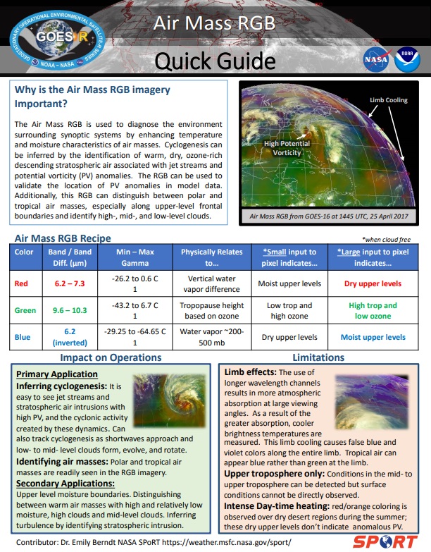
PRÁCTICA 6: CRENDO UNA COMPOSICIÓN RGB (ROJO, VERDE, AZUL)

Creemos una composición RGB Airmass con Python. Considere la receta de Airmass que se encuentra en la Guía rápida de RAMMB:

http://rammb.cira.colostate.edu/training/visit/quick_guides/QuickGuide_GOESR_AirMassRGB_final.pdf

Esta es la receta:

Paso 1) Primeramente, de acuerdo con la receta, necesitamos leer cuatro Bandas GOES-R:

• Banda 08 (6.2 um)
• Banda 10 (7.3 um)
• Banda 12 (9.6 um)
• Banda 13 (10.3 um)

Acceda a la página web de descarga de Amazon del comienzo de este tutorial y descargue los NetCDF’s para la misma fecha y hora para los 4 canales arriba.

http://home.chpc.utah.edu/~u0553130/Brian_Blaylock/cgi-bin/goes16_download.cgi

Esto es lo que deberías tener ahora:

Ya sabemos cómo leer los archivos GOES-R, ¿verdad?

# Open the GOES-R image
file1 = Dataset("OR_ABI-L2-CMIPF-M6C08_G16_s20191981200396_e20191981210104_c20191981210182.nc")
# Get the pixel values, and convert to Celsius
data1 = file1.variables['CMI'][:] - 273.15
#print(data1)

# Open the GOES-R image
file2 = Dataset("OR_ABI-L2-CMIPF-M6C10_G16_s20191981200396_e20191981210116_c20191981210188.nc")
# Get the pixel values, and convert to Celsius
data2 = file2.variables['CMI'][:] - 273.15

# Open the GOES-R image
file3 = Dataset("OR_ABI-L2-CMIPF-M6C12_G16_s20191981200396_e20191981210111_c20191981210185.nc")
# Get the pixel values, and convert to Celsius
data3 = file3.variables['CMI'][:] - 273.15

# Open the GOES-R image
file4 = Dataset("OR_ABI-L2-CMIPF-M6C13_G16_s20191981200396_e20191981210116_c20191981210189.nc")
# Get the pixel values, and convert to Celsius
data4 = file4.variables['CMI'][:] - 273.15

Paso 2) Luego, debemos realizar las operaciones que se ven en la receta (columna central):

# RGB Components
R = data1 - data2
G = data3 - data4
B = data1

Paso 3) Y necesitamos establecer los mínimos, máximos y valores gamma, de acuerdo con la receta:

# Minimuns, Maximuns and Gamma
Rmin = -26.2
Rmax = 0.6

Gmin = -43.2
Gmax = 6.7

Bmin = -29.25
Bmax = -64.65

R[R>Rmax] = Rmax
R[R<Rmin] = Rmin

G[G>Gmax] = Gmax
G[G<Gmin] = Gmin

B[B<Bmax] = Bmax
B[B>Bmin] = Bmin

gamma_R = 1
gamma_G = 1
gamma_B = 1

Paso 4) Normalicemos los datos entre 0 y 1:

# Normalize the data
R = ((R - Rmin) / (Rmax - Rmin)) ** (1/gamma_R)
G = ((G - Gmin) / (Gmax - Gmin)) ** (1/gamma_G)
B = ((B - Bmin) / (Bmax - Bmin)) ** (1/gamma_B)

Paso 5) Finalmente, apilamos los componentes R, G y B para crear el compuesto final:

# Create the RGB
RGB = np.stack([R, G, B], axis=2)

# Eliminate values outside the globe
mask = (RGB == [R[0,0],G[0,0],B[0,0]]).all(axis=2)
RGB[mask] = np.nan

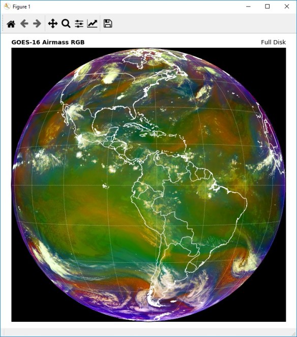
Paso 6) ¡Y haga el plot!

# Choose the plot size (width x height, in inches)
plt.figure(figsize=(7,7))

# Use the Geostationary projection in cartopy
ax = plt.axes(projection=ccrs.Geostationary(central_longitude=-75.0, satellite_height=35786023.0))
img_extent = (-5434894.67527,5434894.67527,-5434894.67527,5434894.67527)

# Add coastlines, borders and gridlines
ax.coastlines(resolution='10m', color='white', linewidth=0.8)
ax.add_feature(cartopy.feature.BORDERS, edgecolor='white', linewidth=0.8)
ax.gridlines(color='white', alpha=0.5, linestyle='--', linewidth=0.5)

# Plot the image
img = ax.imshow(RGB, origin='upper', extent=img_extent)

# Add a title
plt.title('GOES-16 Airmass RGB', fontweight='bold', fontsize=10, loc='left')
plt.title('Full Disk', fontsize=10, loc='right')

# Save the image
plt.tight_layout()
plt.savefig('Image_06.png')

# Show the image
plt.show()

Este debería ser tu script completo por ahora:

# Training: Python and GOES-R Imagery: Script 6

# Required modules
from netCDF4 import Dataset                # Read / Write NetCDF4 files
import matplotlib.pyplot as plt            # Plotting library
import cartopy, cartopy.crs as ccrs        # Plot maps
import numpy as np                         # Import the Numpy packag

# Open the GOES-R image
file1 = Dataset("OR_ABI-L2-CMIPF-M6C08_G16_s20191981200396_e20191981210104_c20191981210182.nc")
# Get the pixel values, and convert to Celsius
data1 = file1.variables['CMI'][:] - 273.15

# Open the GOES-R image
file2 = Dataset("OR_ABI-L2-CMIPF-M6C10_G16_s20191981200396_e20191981210116_c20191981210188.nc")
# Get the pixel values, and convert to Celsius
data2 = file2.variables['CMI'][:] - 273.15

# Open the GOES-R image
file3 = Dataset("OR_ABI-L2-CMIPF-M6C12_G16_s20191981200396_e20191981210111_c20191981210185.nc")
# Get the pixel values, and convert to Celsius
data3 = file3.variables['CMI'][:] - 273.15

# Open the GOES-R image
file4 = Dataset("OR_ABI-L2-CMIPF-M6C13_G16_s20191981200396_e20191981210116_c20191981210189.nc")
# Get the pixel values, and convert to Celsius
data4 = file4.variables['CMI'][:] - 273.15

# RGB Components
R = data1 - data2
G = data3 - data4
B = data1

# Minimuns, Maximuns and Gamma
Rmin = -26.2
Rmax = 0.6

Gmin = -43.2
Gmax = 6.7

Bmin = -29.25
Bmax = -64.65

R[R>Rmax] = Rmax
R[R<Rmin] = Rmin

G[G>Gmax] = Gmax
G[G<Gmin] = Gmin

B[B<Bmax] = Bmax
B[B>Bmin] = Bmin

gamma_R = 1
gamma_G = 1
gamma_B = 1

# Normalize the data
R = ((R - Rmin) / (Rmax - Rmin)) ** (1/gamma_R)
G = ((G - Gmin) / (Gmax - Gmin)) ** (1/gamma_G)
B = ((B - Bmin) / (Bmax - Bmin)) ** (1/gamma_B)

# Create the RGB
RGB = np.stack([R, G, B], axis=2)

# Eliminate values outside the globe
mask = (RGB == [R[0,0],G[0,0],B[0,0]]).all(axis=2)
RGB[mask] = np.nan

# Choose the plot size (width x height, in inches)
plt.figure(figsize=(7,7))

# Use the Geostationary projection in cartopy
ax = plt.axes(projection=ccrs.Geostationary(central_longitude=-75.0, satellite_height=35786023.0))
img_extent = (-5434894.67527,5434894.67527,-5434894.67527,5434894.67527)

# Add coastlines, borders and gridlines
ax.coastlines(resolution='10m', color='white', linewidth=0.8)
ax.add_feature(cartopy.feature.BORDERS, edgecolor='white', linewidth=0.8)
ax.gridlines(color='white', alpha=0.5, linestyle='--', linewidth=0.5)

# Plot the image
img = ax.imshow(RGB, origin='upper', extent=img_extent)

# Add a title
plt.title('GOES-16 Airmass RGB', fontweight='bold', fontsize=10, loc='left')
plt.title('Full Disk', fontsize=10, loc='right')

# Save the image
plt.tight_layout()
plt.savefig('Image_06.png')

# Show the image
plt.show()

PUEDES DESCARGAR EL SCRIPT ARRIBA (Script_06.py) EN ESTE ENLACE

Ejecute el script “Script_06.py” con el siguiente comando:

python Script_06.py

El siguiente plot será creado:

¿Qué puedes cambiar rápidamente en este script?

• Crea un plot de alta resolución. Intente ajustar el scriptpara producir un plot de resolución completa como lo hicimos en el ejercicio 5.
• Agregar shapefiles estados y provincias. Intente agregar shapefiles de estados y provincias como lo hicimos en el ejercicio 5.
• Crea otros RGB. Consulte las Guías Rápidas de RAMMB e intente crear otras RGB. ¡El método de creación DUST RGB es muy similar! ¡Pruébalo! Nota: ¡El canal azul no está invertido!

Hemos terminado los ejercícios de la Introducción al Procesamiento de Imágenes Satelitales con Python!

Siguen abajo algunos scripts extras, para seguir avanzando:

=====================SCRIPTS EXTRAS=====================

SCRIPTS EXTRA 1: SUBPLOTS

SCRIPT EXTRA 1.1: Composición RGB y Componentes R, G y B en el mismo plot

# Training: Python and GOES-R Imagery: RGB Subplots
#---------------------------------------------------------------------------------------------
# Required modules
from netCDF4 import Dataset              # Read / Write NetCDF4 files
import matplotlib.pyplot as plt          # Plotting library
from datetime import datetime, timedelta # Library to convert julian day to dd-mm-yyyy
import cartopy, cartopy.crs as ccrs      # Plot maps
import numpy as np                       # Scientific computing with Python
#---------------------------------------------------------------------------------------------
#---------------------------------------------------------------------------------------------
# Open the GOES-R image
file1 = Dataset("OR_ABI-L2-CMIPF-M6C08_G16_s20191981200396_e20191981210104_c20191981210182.nc")
# Get the pixel values, and convert to Celsius
data1 = file1.variables['CMI'][:] - 273.15

# Open the GOES-R image
file2 = Dataset("OR_ABI-L2-CMIPF-M6C10_G16_s20191981200396_e20191981210116_c20191981210188.nc")
# Get the pixel values, and convert to Celsius
data2 = file2.variables['CMI'][:] - 273.15

# Open the GOES-R image
file3 = Dataset("OR_ABI-L2-CMIPF-M6C12_G16_s20191981200396_e20191981210111_c20191981210185.nc")
# Get the pixel values, and convert to Celsius
data3 = file3.variables['CMI'][:] - 273.15

# Open the GOES-R image
file4 = Dataset("OR_ABI-L2-CMIPF-M6C13_G16_s20191981200396_e20191981210116_c20191981210189.nc")
# Get the pixel values, and convert to Celsius
data4 = file4.variables['CMI'][:] - 273.15
#---------------------------------------------------------------------------------------------
#---------------------------------------------------------------------------------------------
# RGB Components
R = data1 - data2
G = data3 - data4
B = data1

# Minimuns, Maximuns and Gamma
Rmin = -26.2
Rmax = 0.6

Gmin = -43.2
Gmax = 6.7

Bmin = -29.25
Bmax = -64.65

# NOTE: FOR SOME REASON CAN'T PUT GREATER AND LESS THAN SIGNALS ON WORDPRESS
R[R[greater than]Rmax] = Rmax
R[R[less than]Rmin] = Rmin

G[G[greater than]Gmax] = Gmax
G[G[less than]Gmin] = Gmin

B[B[less than]Bmax] = Bmax
B[B[greater than]Bmin] = Bmin 

gamma_R = 1
gamma_G = 1
gamma_B = 1

# Normalize the data
R = ((R - Rmin) / (Rmax - Rmin)) ** (1/gamma_R)
G = ((G - Gmin) / (Gmax - Gmin)) ** (1/gamma_G)
B = ((B - Bmin) / (Bmax - Bmin)) ** (1/gamma_B) 

# Create the RGB
RGB = np.stack([R, G, B], axis=2)

# Eliminate values outside the globe
mask = (RGB == [R[0,0],G[0,0],B[0,0]]).all(axis=2)
RGB[mask] = np.nan
#---------------------------------------------------------------------------------------------
#---------------------------------------------------------------------------------------------
# Choose the plot size (width x height, in inches)
fig, (ax1, ax2, ax3) = plt.subplots(3,2, figsize=(9,7))
#---------------------------------------------------------------------------------------------
#---------------------------------------------------------------------------------------------
# Use the Geostationary projection in cartopy
ax1 = plt.subplot(121,projection=ccrs.Geostationary(central_longitude=-75.0, satellite_height=35786023.0))

# Geostationary extent
img_extent = (-5434894.67527,5434894.67527,-5434894.67527,5434894.67527)

# Eliminate values outside the globe
R[mask] = np.nan

# Plot the image
img1 = ax1.imshow(RGB, origin='upper', extent=img_extent)

# Add coastlines, borders and gridlines
ax1.coastlines(resolution='10m', color='white', linewidth=0.8)
ax1.add_feature(cartopy.feature.BORDERS, edgecolor='white', linewidth=0.5)
ax1.gridlines(color='white', alpha=0.5, linestyle='--', linewidth=0.5, xlocs=np.arange(-180, 180, 15), ylocs=np.arange(-180, 180, 15), draw_labels=False)

# Getting the ABI file date
add_seconds = int(file1.variables['time_bounds'][0])
date = datetime(2000,1,1,12) + timedelta(seconds=add_seconds)
date_format = date.strftime('%B %d %Y - %H:%M UTC')

# Add a title
ax1.set_title('GOES-16 Airmass RGB', fontweight='bold', fontsize=10, loc='left')
ax1.set_title('Full Disk \n' + date_format, fontsize=10, loc='right')
#---------------------------------------------------------------------------------------------
#---------------------------------------------------------------------------------------------
# Use the Geostationary projection in cartopy
ax2 = plt.subplot(322,projection=ccrs.Geostationary(central_longitude=-75.0, satellite_height=35786023.0))

# Geostationary extent
img_extent = (-5434894.67527,5434894.67527,-5434894.67527,5434894.67527)

# Eliminate values outside the globe
G[mask] = np.nan

# Plot the image
img2 = ax2.imshow(R, vmin=0, vmax=1, origin='upper', extent=img_extent, cmap='Reds')

# Add coastlines, borders and gridlines
ax2.coastlines(resolution='10m', color='black', linewidth=0.5)
ax2.add_feature(cartopy.feature.BORDERS, edgecolor='black', linewidth=0.5)
ax2.gridlines(color='black', alpha=0.5, linestyle='--', linewidth=0.5, xlocs=np.arange(-180, 180, 15), ylocs=np.arange(-180, 180, 15), draw_labels=False)

# Add a title
ax2.set_title('Red: 6.2 μm - 7.3 μm', fontweight='bold', fontsize=10, loc='center')
#---------------------------------------------------------------------------------------------
#---------------------------------------------------------------------------------------------
# Use the Geostationary projection in cartopy
ax3 = plt.subplot(324,projection=ccrs.Geostationary(central_longitude=-75.0, satellite_height=35786023.0))

# Geostationary extent
img_extent = (-5434894.67527,5434894.67527,-5434894.67527,5434894.67527)

# Plot the image
img3 = ax3.imshow(G, vmin=0, vmax=1, origin='upper', extent=img_extent, cmap='Greens')

# Add coastlines, borders and gridlines
ax3.coastlines(resolution='10m', color='black', linewidth=0.5)
ax3.add_feature(cartopy.feature.BORDERS, edgecolor='black', linewidth=0.5)
ax3.gridlines(color='black', alpha=0.5, linestyle='--', linewidth=0.5, xlocs=np.arange(-180, 180, 15), ylocs=np.arange(-180, 180, 15), draw_labels=False)

# Add a title
ax3.set_title('Green: 9.6 μm - 10.3 μm', fontweight='bold', fontsize=10, loc='center')
#---------------------------------------------------------------------------------------------
#---------------------------------------------------------------------------------------------
# Use the Geostationary projection in cartopy
ax4 = plt.subplot(326,projection=ccrs.Geostationary(central_longitude=-75.0, satellite_height=35786023.0))

# Geostationary extent
img_extent = (-5434894.67527,5434894.67527,-5434894.67527,5434894.67527)

# Eliminate values outside the globe
B[mask] = np.nan

# Plot the image
img4 = ax4.imshow(B, vmin=0, vmax=1, origin='upper', extent=img_extent, cmap='Blues')

# Add coastlines, borders and gridlines
ax4.coastlines(resolution='10m', color='black', linewidth=0.5)
ax4.add_feature(cartopy.feature.BORDERS, edgecolor='black', linewidth=0.5)
ax4.gridlines(color='black', alpha=0.5, linestyle='--', linewidth=0.5, xlocs=np.arange(-180, 180, 15), ylocs=np.arange(-180, 180, 15), draw_labels=False)

# Add a title
ax4.set_title('Blue: 6.2 μm (inverted)', fontweight='bold', fontsize=10, loc='center')
#---------------------------------------------------------------------------------------------
#---------------------------------------------------------------------------------------------
fig.subplots_adjust(wspace=.01,hspace=.01)
#---------------------------------------------------------------------------------------------
#---------------------------------------------------------------------------------------------
# Automatically adjust subplot parameters
fig.tight_layout()

# Save the image
plt.savefig('Image_13.png')

# Show the image
plt.show()

SCRIPT EXTRA 1.2: Proyección original y cilindrica en el mismo plot

# Training: Python and GOES-R Imagery: Script 8
#---------------------------------------------------------------------------------------------
# Required modules
from netCDF4 import Dataset              # Read / Write NetCDF4 files
import matplotlib.pyplot as plt          # Plotting library
from datetime import datetime, timedelta # Library to convert julian day to dd-mm-yyyy
import cartopy, cartopy.crs as ccrs      # Plot maps
import numpy as np                       # Scientific computing with Python
#---------------------------------------------------------------------------------------------
#---------------------------------------------------------------------------------------------
# Open the GOES-R image
file = Dataset("OR_ABI-L2-CMIPF-M6C13_G16_s20191981200396_e20191981210116_c20191981210189.nc")
# Get the pixel values
data = file.variables['CMI'][:] - 273.15
#---------------------------------------------------------------------------------------------
#---------------------------------------------------------------------------------------------
# Choose the plot size (width x height, in inches)
fig, (ax1, ax2) = plt.subplots(1,2, figsize=(12,7))
#---------------------------------------------------------------------------------------------
#---------------------------------------------------------------------------------------------
# Use the Geostationary projection in cartopy
ax1 = plt.subplot(121,projection=ccrs.Geostationary(central_longitude=-75.0, satellite_height=35786023.0))

# Geostationary extent
img_extent = (-5434894.67527,5434894.67527,-5434894.67527,5434894.67527)

# Plot the image
img1 = ax1.imshow(data, vmin=-80, vmax=40, origin='upper', extent=img_extent, cmap='Greys')

# Add coastlines, borders and gridlines
ax1.coastlines(resolution='10m', color='white', linewidth=0.8)
ax1.add_feature(cartopy.feature.BORDERS, edgecolor='white', linewidth=0.5)
ax1.gridlines(color='white', alpha=0.5, linestyle='--', linewidth=0.5, xlocs=np.arange(-180, 180, 15), ylocs=np.arange(-180, 180, 15), draw_labels=False)

# Add a colorbar
fig.colorbar(img1, label='Brightness Temperature (°C)', extend='both', orientation='horizontal', pad=0.05, fraction=0.05)

# Getting the ABI file date
add_seconds = int(file.variables['time_bounds'][0])
date = datetime(2000,1,1,12) + timedelta(seconds=add_seconds)
date_format = date.strftime('%B %d %Y - %H:%M UTC')

# Add a title
ax1.set_title('GOES-16 (GOES Imager Projection)\nBand 13 (10.35 μm)', fontweight='bold', fontsize=10, loc='left')
ax1.set_title('Full Disk \n' + date_format, fontsize=10, loc='right')

#---------------------------------------------------------------------------------------------
# Use the Geostationary projection in cartopy
ax2 = plt.subplot(122,projection=ccrs.PlateCarree(central_longitude=-75.0))

# Plot Extent
ax2.set_extent([-165.0, 15.0, -90.0, 90.0], crs=ccrs.PlateCarree())

# Add a background image
ax2.stock_img()

# Geostationary extent
img_extent = (-5434894.67527,5434894.67527,-5434894.67527,5434894.67527)

# Plot the image
img2 = ax2.imshow(data, vmin=-80, vmax=40, origin='upper', extent=img_extent, cmap='Greys', transform=ccrs.Geostationary(central_longitude=-75.0))

# Add coastlines, borders and gridlines
ax2.coastlines(resolution='10m', color='white', linewidth=0.8)
ax2.add_feature(cartopy.feature.BORDERS, edgecolor='white', linewidth=0.5)
ax2.gridlines(color='white', alpha=0.5, linestyle='--', linewidth=0.5, xlocs=np.arange(-180, 180, 15), ylocs=np.arange(-180, 180, 15), draw_labels=False)

# Add a colorbar
fig.colorbar(img2, label='Brightness Temperatures (°C)', extend='both', orientation='horizontal', pad=0.05, fraction=0.05)

# Add a title
ax2.set_title('GOES-16 (Cylindrical Projection)\nBand 13 (10.35 μm)', fontweight='bold', fontsize=10, loc='left')
ax2.set_title('Full Disk \n' + date_format, fontsize=10, loc='right')

fig.subplots_adjust(wspace=.02)
#---------------------------------------------------------------------------------------------
#---------------------------------------------------------------------------------------------
# Save the image
plt.savefig('Image_08.png')

# Show the image
plt.show()

SCRIPT EXTRA 1.3: GOES-17 y GOES-16 (proyección geos) en el mismo plot

# Training: Python and GOES-R Imagery: GOES-16 and GOES-17 Subplots
#---------------------------------------------------------------------------------------------
# Required modules
from netCDF4 import Dataset              # Read / Write NetCDF4 files
import matplotlib.pyplot as plt          # Plotting library
from datetime import datetime, timedelta # Library to convert julian day to dd-mm-yyyy
import cartopy, cartopy.crs as ccrs      # Plot maps
import numpy as np                       # Scientific computing with Python
#---------------------------------------------------------------------------------------------
#---------------------------------------------------------------------------------------------
# Open the GOES-R image 1
file1 = Dataset("OR_ABI-L2-CMIPF-M6C13_G17_s20191981200341_e20191981209419_c20191981209474.nc")
# Get the pixel values
data1 = file1.variables['CMI'][:] - 273.15

# Open the GOES-R image 2
file2 = Dataset("OR_ABI-L2-CMIPF-M6C13_G16_s20191981200396_e20191981210116_c20191981210189.nc")
# Get the pixel values
data2 = file2.variables['CMI'][:] - 273.15
#---------------------------------------------------------------------------------------------
#---------------------------------------------------------------------------------------------
# Choose the plot size (width x height, in inches)
fig, (ax1, ax2) = plt.subplots(1,2, figsize=(12,7))
#---------------------------------------------------------------------------------------------
#---------------------------------------------------------------------------------------------
# Use the Geostationary projection in cartopy
ax1 = plt.subplot(121,projection=ccrs.Geostationary(central_longitude=-137.0, satellite_height=35786023.0))
# Geostationary extent
img_extent = (-5434894.67527,5434894.67527,-5434894.67527,5434894.67527)
# Plot the image
img1 = ax1.imshow(data1, vmin=-80, vmax=40, origin='upper', extent=img_extent, cmap='Greys')

# Add coastlines, borders and gridlines
ax1.coastlines(resolution='10m', color='white', linewidth=0.8)
ax1.add_feature(cartopy.feature.BORDERS, edgecolor='white', linewidth=0.5)
ax1.gridlines(color='white', alpha=0.5, linestyle='--', linewidth=0.5, xlocs=np.arange(-180, 180, 15), ylocs=np.arange(-180, 180, 15), draw_labels=False)
# Add a colorbar
fig.colorbar(img1, label='Brightness Temperature (°C)', extend='both', orientation='horizontal', pad=0.05, fraction=0.05)

# Getting the ABI file date
add_seconds = int(file1.variables['time_bounds'][0])
date = datetime(2000,1,1,12) + timedelta(seconds=add_seconds)
date_format = date.strftime('%B %d %Y - %H:%M UTC')

# Add a title
ax1.set_title('GOES-17 Band 13 (10.35 μm)', fontweight='bold', fontsize=10, loc='left')
ax1.set_title('Full Disk \n' + date_format, fontsize=10, loc='right')
#---------------------------------------------------------------------------------------------
# Use the Geostationary projection in cartopy
ax2 = plt.subplot(122,projection=ccrs.Geostationary(central_longitude=-75.0, satellite_height=35786023.0))

# Geostationary extent
img_extent = (-5434894.67527,5434894.67527,-5434894.67527,5434894.67527)

# Plot the image
img2 = ax2.imshow(data2, vmin=-80, vmax=40, origin='upper', extent=img_extent, cmap='Greys')

# Add coastlines, borders and gridlines
ax2.coastlines(resolution='10m', color='white', linewidth=0.8)
ax2.add_feature(cartopy.feature.BORDERS, edgecolor='white', linewidth=0.5)
ax2.gridlines(color='white', alpha=0.5, linestyle='--', linewidth=0.5, xlocs=np.arange(-180, 180, 15), ylocs=np.arange(-180, 180, 15), draw_labels=False)

# Add a colorbar
fig.colorbar(img2, label='Brightness Temperatures (°C)', extend='both', orientation='horizontal', pad=0.05, fraction=0.05)

# Getting the ABI file date
add_seconds = int(file2.variables['time_bounds'][0])
date = datetime(2000,1,1,12) + timedelta(seconds=add_seconds)
date_format = date.strftime('%B %d %Y - %H:%M UTC')

# Add a title
ax2.set_title('GOES-16 Band 13 (10.35 μm)', fontweight='bold', fontsize=10, loc='left')
ax2.set_title('Full Disk \n' + date_format, fontsize=10, loc='right')
#---------------------------------------------------------------------------------------------
#---------------------------------------------------------------------------------------------
fig.subplots_adjust(wspace=.02)
#---------------------------------------------------------------------------------------------
#---------------------------------------------------------------------------------------------
# Save the image
plt.savefig('Image_09.png')

# Show the image
plt.show()

SCRIPT EXTRA 2: GOES-17 Y GOES-16 (MOSAICO) EN EL MISMO PLOT

Un plot muy interesante con un script relativamente simple.

# Training: Python and GOES-R Imagery: Projections

# Required modules
from netCDF4 import Dataset                # Read / Write NetCDF4 files
import matplotlib.pyplot as plt            # Plotting library
import numpy as np                         # Scientific computing with Python
import cartopy, cartopy.crs as ccrs        # Plot maps
from datetime import datetime, timedelta   # Library to convert julian day to dd-mm-yyyy

# Open the GOES-16 image
file1 = Dataset("OR_ABI-L2-CMIPF-M6C13_G16_s20192061900441_e20192061910160_c20192061910249.nc")
# Get the pixel values
data1 = file1.variables['CMI'][:,:] - 273.15
# The projection x and y coordinates equals the scanning angle (in radians) multiplied by the satellite height
sat_h = file1.variables['goes_imager_projection'].perspective_point_height
x1 = file1.variables['x'][:] * sat_h
y1 = file1.variables['y'][:] * sat_h
# Define the image extent
img_extent_1 = (x1.min(), x1.max(), y1.min(), y1.max())

# Open the GOES-17 image
file2 = Dataset("OR_ABI-L2-CMIPF-M6C13_G17_s20192061900341_e20192061909419_c20192061909475.nc")
# Get the pixel values
data2 = file2.variables['CMI'][:,0:4000] - 273.15
# The projection x and y coordinates equals the scanning angle (in radians) multiplied by the satellite height
sat_h = file2.variables['goes_imager_projection'].perspective_point_height
x2 = file2.variables['x'][0:4000] * sat_h
y2 = file2.variables['y'][:] * sat_h
# Define the image extent
img_extent_2 = (x2.min(), x2.max(), y2.min(), y2.max())

# Choose the plot size (width x height, in inches)
plt.figure(figsize=(7,7))

# Plot definition
ax = plt.axes(projection=ccrs.PlateCarree(central_longitude=-103.3))#, globe=globe))
ax.set_extent([-222.0, 10.0, -90.0, 90.0], crs=ccrs.PlateCarree())

# Add a background image
ax.stock_img()

# Add coastlines, borders and gridlines
ax.coastlines(resolution='10m', color='black', linewidth=0.8)
ax.add_feature(cartopy.feature.BORDERS, edgecolor='black', linewidth=0.5)
ax.gridlines(color='gray', alpha=0.5, linestyle='--', linewidth=0.5)

# Plot the image
img = ax.imshow(data1, vmin=-80, vmax=40, origin='upper', extent=img_extent_1, cmap='Greys', transform=ccrs.Geostationary(central_longitude=-75.0, satellite_height=35786023.0))
img = ax.imshow(data2, vmin=-80, vmax=40, origin='upper', extent=img_extent_2, cmap='Greys', transform=ccrs.Geostationary(central_longitude=-137.0, satellite_height=35786023.0))

# Add a colorbar
plt.colorbar(img, label='Brightness Temperatures (°C)', extend='both', orientation='horizontal', pad=0.05, fraction=0.05)

# Getting the file date
add_seconds = int(file2.variables['time_bounds'][0])
date = datetime(2000,1,1,12) + timedelta(seconds=add_seconds)
date = date.strftime('%d %B %Y %H:%M UTC')

# Add a title
plt.title('GOES-16 and GOES-17 Band 13', fontweight='bold', fontsize=10, loc='left')
plt.title('Full Disk \n' + date, fontsize=10, loc='right')

# Save the image
plt.savefig('Image_G16_G17.png')

# Show the image
plt.show()

SCRIPT EXTRA 3: PLOT DE 0.5 KM DE SUB REGIONES DEL FULL DISK

EL PROBLEMA

Las imágenes GOES-16 y GOES-17 de 0,5 km de banda 02 (0,64 um) tienen 21696 x 21696 píxeles, lo que es mucho.

Al crear el plot del disco completo, es necesario una computadora con buenas especificaciones, o tardará mucho tiempo para terminarlo. Pruébalo por ti mismo:

# Training: Python and GOES-R Imagery: Band 02 Full Disk Plot

# Required modules
from netCDF4 import Dataset      # Read / Write NetCDF4 files
import matplotlib.pyplot as plt  # Plotting library

# Open the GOES-R image
file = Dataset("OR_ABI-L2-CMIPF-M6C02_G16_s20192121800485_e20192121810193_c20192121810278.nc")

# Get the pixel values
data = file.variables['CMI'][:]

# Choose the plot size (width x height, in inches)
plt.figure(figsize=(7,7))

# Plot the image
plt.imshow(data, vmin=0, vmax=1.0, cmap='gray')

# Save the image
plt.savefig('Image_VIS.png')

# Show the image
plt.show()

UNA SOLUCIÓN

Una solución es crear el plot solamente para una región determinada del disco completo, seleccionando coordenadas de lat lon específicas en su código.

Así es como debemos proceder para hacerlo:

1-) Convertir las coordenadas GOES-16 en lats y lons (¡solo una vez!) Para usarlas como referencia para indexar cualquier región deseada en discos completos.

Para hacer esto, ejecutaremos el siguiente código una vez, usando una imágen de 2 km para cualquier banda. En el siguiente ejemplo, se utilizó un archivo dela Banda 13. Necesitamos hacer esto solo una vez.

Tenga en cuenta que leeremos cada cuatro píxeles en un archivo de 2 km, por lo que los archivos lat lon de referencia creados tendrán una resolución de 8 km. Podríamos crear archivos de referencia de alta resolución, pero más tarde, tomaría una eternidad leerlos y esa no es la idea. Con pequeños archivos lat lon de referencia de 8 km, se leerán rápidamente cuando sea necesario y proporcionarán una precisión decente para encontrar nuestros índices de 500 m lat lon en el futuro.

from netCDF4 import Dataset                # Read / Write NetCDF4 files
from pyproj import Proj                    # Cartographic projections and coordinate transformations library
import numpy as np                         # Scientific computing with Python

print("Converting G16 coordinates to lons and lats...")

# Reference file
image = "OR_ABI-L2-CMIPF-M6C13_G16_s20192061430442_e20192061440161_c20192061440233.nc"
# Read the file using the NetCDF library
file = Dataset(image)
# Satellite height
sat_h = file.variables['goes_imager_projection'].perspective_point_height
# Satellite longitude
sat_lon = file.variables['goes_imager_projection'].longitude_of_projection_origin
# Satellite sweep
sat_sweep = file.variables['goes_imager_projection'].sweep_angle_axis
# The projection x and y coordinates equals
# the scanning angle (in radians) multiplied by the satellite height (http://proj4.org/projections/geos.html)
X = file.variables['x'][:][::4] * sat_h
Y = file.variables['y'][:][::4] * sat_h
# map object with pyproj
p = Proj(proj='geos', h=sat_h, lon_0=sat_lon, sweep=sat_sweep, a=6378137.0)
# Convert map points to latitude and longitude with the magic provided by Pyproj
XX, YY = np.meshgrid(X, Y)
lons, lats = p(XX, YY, inverse=True)

# Pixels outside the globe as -9999
mask = (lons == lons[0][0])
lons[mask] = -9999
lats[mask] = -9999

print("Saving lat long arrays for later use...")
np.savetxt('g16_lons_8km.txt', lons, fmt='%.2f')
np.savetxt('g16_lats_8km.txt', lats, fmt='%.2f')

Al ejecutar este código, se crearán dos archivos:

• g16_lons_8km.txt
• g16_lats_8km.txt

Ya no es necesario ejecutar este código, pues ya creastes la referencia.

En lugar de ejecutar este código, puede descargar los archivos de referencia en los siguientes enlaces:

• g16_lats_8km.txt
• g16_lons_8km.txt

2-) Use los archivos lat lon de referencia para seleccionar solo una región determinada del disco completo

Ok, ahora que tenemos nuestros archivos de referencia de lat lon, podemos usarlos para leer cualquier banda GOES-16 para cualquier región específica que queramos en la proyección original, con una buena precisión de lat lon. Esto hará que los plots sean mucho más rápidos.

Supongamos que queremos crear el plot de un archivo Band 02 de 0.5 km:

# Open the GOES-R image
file = Dataset("OR_ABI-L2-CMIPF-M6C02_G16_s20192121800485_e20192121810193_c20192121810278.nc")

Y queremos crear el plot solo para la siguiente región aproximada:

• Min lon: -74.0
• Max lon: -66.0
• Min lat: -21.0
• Max lat: -14.0

# Desired visualization extent [min_lon, max_lon, min_lat, max_lat]
min_lon, max_lon, min_lat, max_lat = -74.0, -66.0, -21.0, -14.0
extent = [min_lon, min_lat, max_lon, max_lat]

Leamos nuestros archivos lat lon de referencia como matrices numpy:

# Read the GOES-R lat lons as arrays (files created previously)
lons = np.loadtxt('g16_lons_8km.txt')
lats = np.loadtxt('g16_lats_8km.txt')
ref_grid_resolution_km = 8

DONDE OCURRE LA MAGIA

El siguiente fragmento de código encuentra los índices de pares de píxeles que mejor coinciden con los lat lat que queremos:

# Calculate the lat lon pairs indexes for the desired extent
idx_pair_1 = abs(lats-extent[1])+abs(lons-extent[0])
max_lat_idx,min_lon_idx = np.unravel_index(idx_pair_1.argmin(),idx_pair_1.shape)
idx_pair_2 = abs(lats-extent[3])+abs(lons-extent[2])
min_lat_idx,max_lon_idx = np.unravel_index(idx_pair_2.argmin(),idx_pair_2.shape)

# Adapt the reference indexes for the current file resolution
min_lat_idx = min_lat_idx * int(ref_grid_resolution_km/band_resolution_km)
min_lon_idx = min_lon_idx * int(ref_grid_resolution_km/band_resolution_km)
max_lat_idx = max_lat_idx * int(ref_grid_resolution_km/band_resolution_km)
max_lon_idx = max_lon_idx * int(ref_grid_resolution_km/band_resolution_km)

Entonces, solo leemos estos píxeles de nuestro enorme archivo de 500 m:

# Get the pixel values
data = file.variables['CMI'][min_lat_idx:max_lat_idx,min_lon_idx:max_lon_idx][::1,::1]

Este es nuestro ejemplo completo:

# Training: Python and GOES-R Imagery: Read 500 m faster

# Required modules
from netCDF4 import Dataset                # Read / Write NetCDF4 files
import matplotlib.pyplot as plt            # Plotting library
import numpy as np                         # Scientific computing with Python
import cartopy, cartopy.crs as ccrs        # Plot maps
import cartopy.io.shapereader as shpreader # Import shapefiles
from datetime import datetime, timedelta   # Library to convert julian day to dd-mm-yyyy

# Open the GOES-R image
file = Dataset("OR_ABI-L2-CMIPF-M6C02_G16_s20192121800485_e20192121810193_c20192121810278.nc")

# Get the image resolution
band_resolution_km = getattr(file, 'spatial_resolution')
band_resolution_km = float(band_resolution_km[:band_resolution_km.find("km")])

# Desired visualization extent [min_lon, max_lon, min_lat, max_lat]
#min_lon, max_lon, min_lat, max_lat = -60.0, -34.0, -30.0, -15.0
min_lon, max_lon, min_lat, max_lat = -74.0, -66.0, -21.0, -14.0
extent = [min_lon, min_lat, max_lon, max_lat]

# Read the GOES-R lat lons as arrays (files created previously)
lons = np.loadtxt('g16_lons_8km.txt')
lats = np.loadtxt('g16_lats_8km.txt')
ref_grid_resolution_km = 8

# Calculate the lat lon pairs indexes for the desired extent
idx_pair_1 = abs(lats-extent[1])+abs(lons-extent[0])
max_lat_idx,min_lon_idx = np.unravel_index(idx_pair_1.argmin(),idx_pair_1.shape)
idx_pair_2 = abs(lats-extent[3])+abs(lons-extent[2])
min_lat_idx,max_lon_idx = np.unravel_index(idx_pair_2.argmin(),idx_pair_2.shape)

# Adapt the reference indexes for the current file resolution
min_lat_idx = min_lat_idx * int(ref_grid_resolution_km/band_resolution_km)
min_lon_idx = min_lon_idx * int(ref_grid_resolution_km/band_resolution_km)
max_lat_idx = max_lat_idx * int(ref_grid_resolution_km/band_resolution_km)
max_lon_idx = max_lon_idx * int(ref_grid_resolution_km/band_resolution_km)

# The projection x and y coordinates equals the scanning angle (in radians) multiplied by the satellite height
sat_h = file.variables['goes_imager_projection'].perspective_point_height
x = file.variables['x'][min_lon_idx:max_lon_idx] * sat_h
y = file.variables['y'][min_lat_idx:max_lat_idx] * sat_h

# Get the pixel values
data = file.variables['CMI'][min_lat_idx:max_lat_idx,min_lon_idx:max_lon_idx][::1,::1]

# Choose the plot size (width x height, in inches)
plt.figure(figsize=(7,7))

# Use the Geostationary projection in cartopy
ax = plt.axes(projection=ccrs.Geostationary(central_longitude=-75.0, satellite_height=35786023.0))
img_extent = (x.min(), x.max(), y.min(), y.max())

# Add a shapefile
shapefile = list(shpreader.Reader('ne_10m_admin_1_states_provinces.shp').geometries())
ax.add_geometries(shapefile, ccrs.PlateCarree(), edgecolor='gold',facecolor='none', linewidth=0.3)

# Add coastlines, borders and gridlines
ax.coastlines(resolution='10m', color='white', linewidth=0.8)
#ax.add_feature(cartopy.feature.BORDERS, edgecolor='gray', linewidth=1.0)
ax.gridlines(color='white', alpha=0.5, linestyle='--', linewidth=0.5)

# Inserting City Labels
city_lons = [-69.3013, -67.8007]
city_lats = [-15.8993, -20.2443]
labels = ['Lake Titicaca', 'Salar de Uyuni']
x_offsets = [0.1,0.1]
y_offsets = [0,0]

ax.plot(city_lons, city_lats, 'bo', color='cyan', markersize=5, transform=ccrs.Geodetic())

for label, xpt, ypt, x_offset, y_offset in zip(labels, city_lons, city_lats, x_offsets, y_offsets):
ax.text(xpt+x_offset , ypt+y_offset, label, fontsize=12, fontweight='bold', zorder=8, color='gold', transform=ccrs.Geodetic())

# Plot the image
img = ax.imshow(data, vmin=0.0, vmax=0.7, extent=img_extent, origin='upper', cmap='gray')

# Getting the file date
add_seconds = int(file.variables['time_bounds'][0])
date = datetime(2000,1,1,12) + timedelta(seconds=add_seconds)
date = date.strftime('%d %B %Y %H:%M UTC')

# Add a title
plt.title('GOES-16 Band 02 (500m)', fontweight='bold', fontsize=10, loc='left')
plt.title('Sub Region \n' + date, fontsize=10, loc='right')

# Save the image
plt.savefig('Image_08.png')

# Show the image
plt.show()

Este script va a ejecutarse muy rapidamente….

Genial no?

Última actualización en 19 de Agosto de 2019, 15:00 UTC

Amazing stuff with a relatively simple script…

# Training: Python and GOES-R Imagery: Projections

# Required modules
from netCDF4 import Dataset                # Read / Write NetCDF4 files
import matplotlib.pyplot as plt            # Plotting library
import numpy as np                         # Scientific computing with Python
import cartopy, cartopy.crs as ccrs        # Plot maps
from datetime import datetime, timedelta   # Library to convert julian day to dd-mm-yyyy

# Open the GOES-16 image
file1 = Dataset("OR_ABI-L2-CMIPF-M6C13_G16_s20192061900441_e20192061910160_c20192061910249.nc")
# Get the pixel values
data1 = file1.variables['CMI'][:,:] - 273.15
# The projection x and y coordinates equals the scanning angle (in radians) multiplied by the satellite height
sat_h = file1.variables['goes_imager_projection'].perspective_point_height
x1 = file1.variables['x'][:] * sat_h
y1 = file1.variables['y'][:] * sat_h
# Define the image extent
img_extent_1 = (x1.min(), x1.max(), y1.min(), y1.max())

# Open the GOES-17 image
file2 = Dataset("OR_ABI-L2-CMIPF-M6C13_G17_s20192061900341_e20192061909419_c20192061909475.nc")
# Get the pixel values
data2 = file2.variables['CMI'][:,0:4000] - 273.15
# The projection x and y coordinates equals the scanning angle (in radians) multiplied by the satellite height
sat_h = file2.variables['goes_imager_projection'].perspective_point_height
x2 = file2.variables['x'][0:4000] * sat_h
y2 = file2.variables['y'][:] * sat_h
# Define the image extent
img_extent_2 = (x2.min(), x2.max(), y2.min(), y2.max())

# Choose the plot size (width x height, in inches)
plt.figure(figsize=(7,7))

# Plot definition
ax = plt.axes(projection=ccrs.PlateCarree(central_longitude=-103.3))#, globe=globe))
ax.set_extent([-222.0, 10.0, -90.0, 90.0], crs=ccrs.PlateCarree())

# Add a background image
ax.stock_img()

# Add coastlines, borders and gridlines
ax.coastlines(resolution='10m', color='black', linewidth=0.8)
ax.add_feature(cartopy.feature.BORDERS, edgecolor='black', linewidth=0.5)
ax.gridlines(color='gray', alpha=0.5, linestyle='--', linewidth=0.5)

# Plot the image
img = ax.imshow(data1, vmin=-80, vmax=40, origin='upper', extent=img_extent_1, cmap='Greys', transform=ccrs.Geostationary(central_longitude=-75.0, satellite_height=35786023.0))
img = ax.imshow(data2, vmin=-80, vmax=40, origin='upper', extent=img_extent_2, cmap='Greys', transform=ccrs.Geostationary(central_longitude=-137.0, satellite_height=35786023.0))

# Add a colorbar
plt.colorbar(img, label='Brightness Temperatures (°C)', extend='both', orientation='horizontal', pad=0.05, fraction=0.05)

# Getting the file date
add_seconds = int(file2.variables['time_bounds'][0])
date = datetime(2000,1,1,12) + timedelta(seconds=add_seconds)
date = date.strftime('%d %B %Y %H:%M UTC')

# Add a title
plt.title('GOES-16 and GOES-17 Band 13', fontweight='bold', fontsize=10, loc='left')
plt.title('Full Disk \n' + date, fontsize=10, loc='right')

# Save the image
plt.savefig('Image_G16_G17.png')

# Show the image
plt.show()

Hi all,

THE PROBLEM

GOES-16 and GOES-17 0.5 km Band 02 (0.64 um) imagery has 21696 x 21696 pixels, which is a lot.

When plotting the full disk, you need a computer with good specs, or it will take loooong minutes to finish it. Try it for yourself:

# Training: Python and GOES-R Imagery: Band 02 Full Disk Plot

# Required modules
from netCDF4 import Dataset      # Read / Write NetCDF4 files
import matplotlib.pyplot as plt  # Plotting library

# Open the GOES-R image
file = Dataset("OR_ABI-L2-CMIPF-M6C02_G16_s20192121800485_e20192121810193_c20192121810278.nc")

# Get the pixel values
data = file.variables['CMI'][:]

# Choose the plot size (width x height, in inches)
plt.figure(figsize=(7,7))

# Plot the image
plt.imshow(data, vmin=0, vmax=1.0, cmap='gray')

# Save the image
plt.savefig('Image_VIS.png')

# Show the image
plt.show()

A SOLUTION

One solution is to plot only a given region of the Full Disk, selecting specific lat lon coordinates in your code.

This is how we should proceed in order to do it:

1-) Convert GOES-16 coordinates to lats and lons (only once!) in order to use them as a reference to index any desired region in Full Disks.

To do this, we’ll run the following code once, using any 2 km imagery for any band. In the example below a Band 13 file was used. We need to do this only once.

Please note that we’ll read every four pixels in a 2 km file, so the created reference lat lon files will have an 8 km resolution. We could create higher resolution lat lon reference files but later, it would take an eternity to read them and that’s not the idea. With small 8 km reference lat lon files, they would be quickly read when needed and would provide a decent precision in order to find our 500 m lat lon indexes in the future.

from netCDF4 import Dataset                # Read / Write NetCDF4 files
from pyproj import Proj                    # Cartographic projections and coordinate transformations library
import numpy as np                         # Scientific computing with Python

print("Converting G16 coordinates to lons and lats...")

# Reference file
image = "OR_ABI-L2-CMIPF-M6C13_G16_s20192061430442_e20192061440161_c20192061440233.nc"
# Read the file using the NetCDF library
file = Dataset(image)
# Satellite height
sat_h = file.variables['goes_imager_projection'].perspective_point_height
# Satellite longitude
sat_lon = file.variables['goes_imager_projection'].longitude_of_projection_origin
# Satellite sweep
sat_sweep = file.variables['goes_imager_projection'].sweep_angle_axis
# The projection x and y coordinates equals
# the scanning angle (in radians) multiplied by the satellite height (http://proj4.org/projections/geos.html)
X = file.variables['x'][:][::4] * sat_h
Y = file.variables['y'][:][::4] * sat_h
# map object with pyproj
p = Proj(proj='geos', h=sat_h, lon_0=sat_lon, sweep=sat_sweep, a=6378137.0)
# Convert map points to latitude and longitude with the magic provided by Pyproj
XX, YY = np.meshgrid(X, Y)
lons, lats = p(XX, YY, inverse=True)

# Pixels outside the globe as -9999
mask = (lons == lons[0][0])
lons[mask] = -9999
lats[mask] = -9999

print("Saving lat long arrays for later use...")
np.savetxt('g16_lons_8km.txt', lons, fmt='%.2f')
np.savetxt('g16_lats_8km.txt', lats, fmt='%.2f')

When running this code, two files will be created:

• g16_lons_8km.txt
• g16_lats_8km.txt

You don’t need to run this code anymore.

Instead of running this code, you may download the reference files at the following links:

• g16_lats_8km.txt
• g16_lons_8km.txt

2-) Use the reference lat lon files to select only a given region of the full disk

Ok, now that we have our lat lon reference files, we may use them to read any GOES-16 Band for any specific region we want in the original projection, with a good lat lon accuracy. This will make the plots much faster.

Suppose we want to plot a 0.5 km Band 02 file:

# Open the GOES-R image
file = Dataset("OR_ABI-L2-CMIPF-M6C02_G16_s20192121800485_e20192121810193_c20192121810278.nc")

And we wan’t to plot it only for the following approximate region:

• Min lon: -74.0
• Max lon: -66.0
• Min lat: -21.0
• Max lat: -14.0

# Desired visualization extent [min_lon, max_lon, min_lat, max_lat]
min_lon, max_lon, min_lat, max_lat = -74.0, -66.0, -21.0, -14.0
extent = [min_lon, min_lat, max_lon, max_lat]

Let’s read our reference lat lon files as numpy arrays:

# Read the GOES-R lat lons as arrays (files created previously)
lons = np.loadtxt('g16_lons_8km.txt')
lats = np.loadtxt('g16_lats_8km.txt')
ref_grid_resolution_km = 8

WHERE THE MAGIC HAPPENS

The following piece of code finds the pixel pairs indexes that better matches the lat lons we want:

# Calculate the lat lon pairs indexes for the desired extent
idx_pair_1 = abs(lats-extent[1])+abs(lons-extent[0])
max_lat_idx,min_lon_idx = np.unravel_index(idx_pair_1.argmin(),idx_pair_1.shape)
idx_pair_2 = abs(lats-extent[3])+abs(lons-extent[2])
min_lat_idx,max_lon_idx = np.unravel_index(idx_pair_2.argmin(),idx_pair_2.shape)

# Adapt the reference indexes for the current file resolution
min_lat_idx = min_lat_idx * int(ref_grid_resolution_km/band_resolution_km)
min_lon_idx = min_lon_idx * int(ref_grid_resolution_km/band_resolution_km)
max_lat_idx = max_lat_idx * int(ref_grid_resolution_km/band_resolution_km)
max_lon_idx = max_lon_idx * int(ref_grid_resolution_km/band_resolution_km)

So, we only read these pixels from our huge 500 m file:

# Get the pixel values
data = file.variables['CMI'][min_lat_idx:max_lat_idx,min_lon_idx:max_lon_idx][::1,::1]

This is our full code example:

# Training: Python and GOES-R Imagery: Read 500 m faster

# Required modules
from netCDF4 import Dataset                # Read / Write NetCDF4 files
import matplotlib.pyplot as plt            # Plotting library
import numpy as np                         # Scientific computing with Python
import cartopy, cartopy.crs as ccrs        # Plot maps
import cartopy.io.shapereader as shpreader # Import shapefiles
from datetime import datetime, timedelta   # Library to convert julian day to dd-mm-yyyy

# Open the GOES-R image
file = Dataset("OR_ABI-L2-CMIPF-M6C02_G16_s20192121800485_e20192121810193_c20192121810278.nc")

# Get the image resolution
band_resolution_km = getattr(file, 'spatial_resolution')
band_resolution_km = float(band_resolution_km[:band_resolution_km.find("km")])

# Desired visualization extent [min_lon, max_lon, min_lat, max_lat]
#min_lon, max_lon, min_lat, max_lat = -60.0, -34.0, -30.0, -15.0
min_lon, max_lon, min_lat, max_lat = -74.0, -66.0, -21.0, -14.0
extent = [min_lon, min_lat, max_lon, max_lat]

# Read the GOES-R lat lons as arrays (files created previously)
lons = np.loadtxt('g16_lons_8km.txt')
lats = np.loadtxt('g16_lats_8km.txt')
ref_grid_resolution_km = 8

# Calculate the lat lon pairs indexes for the desired extent
idx_pair_1 = abs(lats-extent[1])+abs(lons-extent[0])
max_lat_idx,min_lon_idx = np.unravel_index(idx_pair_1.argmin(),idx_pair_1.shape)
idx_pair_2 = abs(lats-extent[3])+abs(lons-extent[2])
min_lat_idx,max_lon_idx = np.unravel_index(idx_pair_2.argmin(),idx_pair_2.shape)

# Adapt the reference indexes for the current file resolution
min_lat_idx = min_lat_idx * int(ref_grid_resolution_km/band_resolution_km)
min_lon_idx = min_lon_idx * int(ref_grid_resolution_km/band_resolution_km)
max_lat_idx = max_lat_idx * int(ref_grid_resolution_km/band_resolution_km)
max_lon_idx = max_lon_idx * int(ref_grid_resolution_km/band_resolution_km)

# The projection x and y coordinates equals the scanning angle (in radians) multiplied by the satellite height
sat_h = file.variables['goes_imager_projection'].perspective_point_height
x = file.variables['x'][min_lon_idx:max_lon_idx] * sat_h
y = file.variables['y'][min_lat_idx:max_lat_idx] * sat_h

# Get the pixel values
data = file.variables['CMI'][min_lat_idx:max_lat_idx,min_lon_idx:max_lon_idx][::1,::1]

# Choose the plot size (width x height, in inches)
plt.figure(figsize=(7,7))

# Use the Geostationary projection in cartopy
ax = plt.axes(projection=ccrs.Geostationary(central_longitude=-75.0, satellite_height=35786023.0))
img_extent = (x.min(), x.max(), y.min(), y.max())

# Add a shapefile
shapefile = list(shpreader.Reader('ne_10m_admin_1_states_provinces.shp').geometries())
ax.add_geometries(shapefile, ccrs.PlateCarree(), edgecolor='gold',facecolor='none', linewidth=0.3)

# Add coastlines, borders and gridlines
ax.coastlines(resolution='10m', color='white', linewidth=0.8)
#ax.add_feature(cartopy.feature.BORDERS, edgecolor='gray', linewidth=1.0)
ax.gridlines(color='white', alpha=0.5, linestyle='--', linewidth=0.5)

# Inserting City Labels
city_lons = [-69.3013, -67.8007]
city_lats = [-15.8993, -20.2443]
labels = ['Lake Titicaca', 'Salar de Uyuni']
x_offsets = [0.1,0.1]
y_offsets = [0,0]

ax.plot(city_lons, city_lats, 'bo', color='cyan', markersize=5, transform=ccrs.Geodetic())

for label, xpt, ypt, x_offset, y_offset in zip(labels, city_lons, city_lats, x_offsets, y_offsets):
ax.text(xpt+x_offset , ypt+y_offset, label, fontsize=12, fontweight='bold', zorder=8, color='gold', transform=ccrs.Geodetic())

# Plot the image
img = ax.imshow(data, vmin=0.0, vmax=0.7, extent=img_extent, origin='upper', cmap='gray')

# Getting the file date
add_seconds = int(file.variables['time_bounds'][0])
date = datetime(2000,1,1,12) + timedelta(seconds=add_seconds)
date = date.strftime('%d %B %Y %H:%M UTC')

# Add a title
plt.title('GOES-16 Band 02 (500m)', fontweight='bold', fontsize=10, loc='left')
plt.title('Sub Region \n' + date, fontsize=10, loc='right')

# Save the image
plt.savefig('Image_08.png')

# Show the image
plt.show()

This script will run very fast….

Great isn’t it?