Hi community!

On 2017, we have seen on this post a nice web interface developed by Brian Blaylock to download GOES-R imagery from the cloud. On 2018,  Dr. Marcial Garbanzo from the University of Costa Rica kindly shared a Shell script example to do the same, routinely.

Back on October 2018 Brian created a nice tutorial on how to do it using Python and a command line program called Rclone.

As he says:

As part of NOAA’s Big Data Project, Amazon makes available NEXRAD, GOES, and other data publicly available via Amazon Web Services (AWS). You can use rclone to access this data and download for your use. (You can even use rclone to access personal OneDrive, Google Drive, Box, and other types of cloud storage.)

Check out on this web page the public data available on AWS. It includes GOES-16, GOES-17, NEXRAD, Sentinel-1, Sentinel-2, Landsat 8, MODIS, CBERS, GFS, and many other.

In this blog series, we’ll try to learn how to use Rclone with Python so we may easily acess these public datasets.

For the GNC-A users, this could be really useful, because they could download the remaining GOES-R bands that are not on the broadcast (01, 03, 04, 05, 06, 10, 11, 12 and 16), or the full disks from minutes 20 and 50.

First of all, let’s learn how to use Rclone without Python.

LEARNING TO USE THE RCLONE COMMAND LINE TOOL

1 – Download and install Rclone in your machine. In this example we’ll use a Windows machine, so we simply extracted the “rclone.exe” in a folder at “C:\Rclone”.

2 – In our examples, we’ll use only three basic Rclone commands:

• List directories (rclone lsd) 
• List files (rclone ls)
• Copy files (rclone copy)

Listing Directories

3 – Let’s see how we can list the available directories for GOES-16/17. The basic command structure is as follows:

 rclone.exe lsd publicAWS:BUCKET/PRODUCT/YEAR/JULIANDAY/

Note: When using rclone in other operational systems, the “.exe” is not needed.

Where:

BUCKET:

noaa-goes16 or noaa-goes17 (or any other public dataset)

Let’s check the available products for GOES-16 using the following command:

 rclone.exe lsd publicAWS:noaa-goes16/

This should be the output:

Where:

PRODUCT:

• ABI-L1b-RadC: Level 1b Radiances (CONUS)
• ABI-L1b-RadF: Level 1b Radiances (Full-Disk)
• ABI-L1b-RadM: Level 1b Radiances (Mesoscale)
• ABI-L2-CMIPC: Level 2 CMI (CONUS)
• ABI-L2-CMIPF: Level 2 CMI (Full-Disk)
• ABI-L2-CMIPM: Level 2 CMI (Mesoscale)
• ABI-L2-MCMIPC: Level 2 CMI (CONUS) – All 16 bands [2 km] in a single NetCDF file.
• ABI-L2-MCMIPF: Level 2 CMI (Full-Disk) – All 16 bands [2 km] in a single NetCDF  file.
• ABI-L2-MCMIPM: Level 2 CMI (Mesoscale) – All 16 bands [2 km] in a single NetCDF file.

Let’s check the available times for the ABI-L2-CMIPF files for today (April 12, 2019). You may check the Julian Day here:

• YEAR: 2019
• JULIANDAY: 102

So, let’s use the following command:

 rclone.exe lsd publicAWS:noaa-goes16/ABI-L2-CMIPF/2019/102/

Right now is 13:55 UTC, and this was the output:

Hour 13 UTC is the most recent directory available.

Listing Files

4 – Let’s see how we can list the available files inside this directory, using the ls Rclone command (not lsd!):

 rclone.exe ls publicAWS:BUCKET/PRODUCT/YEAR/JULIANDAY/HOUR/

rclone.exe ls publicAWS:noaa-goes16/ABI-L2-CMIPF/2019/102/13/

This was the output (the image doesn’t show not all files listed):

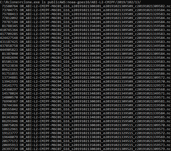
The list shows the file sizes in bytes and the file names. All GOES-16 channels are listed togheter.

Downloading Files

5 – Now that we have the files listed, let’s download one of them with the copy Rclone command, using the following command structure:

rclone.exe copy publicAWS:BUCKET/PRODUCT/YEAR/JULIANDAY/HOUR/FILE OUTDIR

Where:

• FILE: NetCDF file to download
• OUTDIR: Directory in your local machine where the file will be stored

Let’s download the following file:

And copy it the the same directory where we have the RClone executable (C:\Rclone\)

rclone.exe copy publicAWS:noaa-goes16/ABI-L2-CMIPF/2019/102/13/OR_ABI-L2-CMIPF-M6C16_G16_s20191021350201_e20191021359521_c20191021359598.nc C:\Rclone\

After a while, you should see the downloaded file in the selected directory:

Now that we have learned the basics of the Rclone tool, let’s see how we can use it with Python.

USING RCLONE WITH PYTHON – A FIRST APPROACH

Listing Directories With Python

1 – For this example, we created a rclone_tutorial_1.py script in the same directory where we have the rclone tool:

First of all, let’s see how we can list the available products again, now with Python:

rclone.exe lsd publicAWS:BUCKET/

As seen on the tutorial from Brian, let’s use the following Python code:

# Required Modules
import subprocess
# The subprocess module allows you to spawn new processes, connect to their input/output/error pipes, and obtain their return codes.
# Get output from rclone command
files = subprocess.check_output('rclone.exe lsd publicAWS:noaa-goes16/', shell=True)
# Change type from 'bytes' to 'string'
files = files.decode()
# Split files based on the new line and remove the empty item at the end.
files = files.split('\n')
files.remove('')
# Print the list of directories
for i in files:
    print(i)

When executing the script (python rclone_tutorial_1.py), this shoud be the output:

Listing Files With Python

2 – Let’s see how we can list the available files inside this directory, using the ls Rclone command (not lsd!) again, now with Python:

 rclone.exe ls publicAWS:BUCKET/PRODUCT/YEAR/JULIANDAY/HOUR/

rclone.exe ls publicAWS:noaa-goes16/ABI-L2-CMIPF/2019/102/13/

Let’s change our script in the following line:

# Get output from rclone command
files = subprocess.check_output('rclone.exe ls publicAWS:noaa-goes16/ABI-L2-CMIPF/2019/102/13/', shell=True)

When executing the script, this shoud be the output:

Ok, so let’s download a file now.

Downloading Files With Python

3 – Let’s download one of them with the copy Rclone command, now using Python, with the following command:

rclone.exe copy publicAWS:noaa-goes16/ABI-L2-CMIPF/2019/102/13/OR_ABI-L2-CMIPF- M6C13_G16_s20191021350201_e20191021359521_c20191021359599.nc C:\Rclone\

Note: We have changed the example file to Band13 now.

To download the example file, let’s use the following Python code:

# Required Modules
import os # Miscellaneous operating system interfaces
# Download the most recent file to the specified directory
os.system('rclone.exe copy publicAWS:noaa-goes16/ABI-L2-CMIPF/2019/102/13/OR_ABI-L2-CMIPF-M6C13_G16_s20191021350201_e20191021359521_c20191021359599.nc C:\\Rclone\\')

After executing the script, this shoud see the new file downloaded in the directory:

Now that we have seen the basic commands with Python, let’s change our code a little bit.

USING RCLONE WITH PYTHON – A SECOND APPROACH

In the previous script examples, we manually indicated the full Rclone command in the Python code:

files = subprocess.check_output('rclone.exe ls publicAWS:noaa-goes16/ABI-L2-CMIPF/2019/102/13/', shell=True)

os.system('rclone.exe copy publicAWS:noaa-goes16/ABI-L2-CMIPF/2019/102/13/OR_ABI-L2-CMIPF-M6C13_G16_s20191021350201_e20191021359521_c20191021359599.nc C:\\Rclone\\')

 

Let’s make the code more useful, little by little:

Adding variables

Considering that our Rclone command is:

 rclone.exe COMMAND publicAWS:BUCKET/PRODUCT/YEAR/JULIANDAY/HOUR/FILE OUTDIR

Let’s create variables for BUCKET, PRODUCT, YEAR, JULIANDAY and HOUR, and list the available files for a random year, day and hour, using the following code:

# Required Modules
import os           # Miscellaneous operating system interfaces
import subprocess   # The subprocess module allows you to spawn new processes, connect to their input/output/error pipes, and obtain their return codes.

# Desired Data
BUCKET = 'noaa-goes16'    # For GOES-R the buckets are: ['noaa-goes16', 'noaa-goes17']
PRODUCT = 'ABI-L2-CMIPF'  # Choose from ['ABI-L1b-RadC', 'ABI-L1b-RadF', 'ABI-L1b-RadM', 'ABI-L2-CMIPC', 'ABI-L2-CMIPF', 'ABI-L2-CMIPM', 'ABI-L2-MCMIPC', 'ABI-L2-MCMIPF', 'ABI-L2-MCMIPM']
YEAR = '2018'             # Choose from ['2017', '2018', '2019']
JULIAN_DAY = '102'        # Data available after julian day 283, 2017 (October 10, 2017)
HOUR = '12'               # Choose from 00 to 23 

# Get output from rclone command, based on the desired data
files = subprocess.check_output('rclone.exe' + " " + 'ls publicAWS:' + BUCKET + "/" + PRODUCT + "/" + YEAR + "/" + JULIAN_DAY + "/" + HOUR + "/", shell=True)
# Change type from 'bytes' to 'string'
files = files.decode()
# Split files based on the new line and remove the empty item at the end.
files = files.split('\n')
files.remove('')
# Print the file names list
for i in files:
    print(i)

The output should show the files for 2018, julian day 102 and 12 UTC (not all files are shown in the image below):

Listing only a given channel and making the code work on both Windows and Linux

Remeber in the beggining of the tutorial we saying that when using rclone in other operational systems, the “.exe” is not needed? Let’s add that to the code:

import platform           # Access to underlying platform’s identifying data
osystem = platform.system()    # Get the O.S.
if osystem == "Windows": extension = '.exe'

# Get output from rclone command, based on the desired data
files = subprocess.check_output('rclone' + extension + " " + 'ls publicAWS:' + BUCKET + "/" + PRODUCT + "/" + YEAR + "/" + JULIAN_DAY + "/" + HOUR + "/", shell=True)

Also, let’s create a CHANNEL variable:

CHANNEL = 'C13'           # Choose from ['C01 C02 C03 C04 C05 C06 C07 C08 C09 C10 C11 C12 C13 C14 C15 C16']

And list only the available files for a given channel:

# Get only the file names for an specific channel
files = [x for x in files if CHANNEL in x ]

Now our full script is:

# Required Modules
import os           # Miscellaneous operating system interfaces
import subprocess   # The subprocess module allows you to spawn new processes, connect to their input/output/error pipes, and obtain their return codes.
import platform     # Access to underlying platform’s identifying data
osystem = platform.system()
if osystem == "Windows": extension = '.exe'

# Desired Data
BUCKET = 'noaa-goes16'    # For GOES-R the buckets are: ['noaa-goes16', 'noaa-goes17']
PRODUCT = 'ABI-L2-CMIPF'  # Choose from ['ABI-L1b-RadC', 'ABI-L1b-RadF', 'ABI-L1b-RadM', 'ABI-L2-CMIPC', 'ABI-L2-CMIPF', 'ABI-L2-CMIPM', 'ABI-L2-MCMIPC', 'ABI-L2-MCMIPF', 'ABI-L2-MCMIPM']
YEAR = '2018'             # Choose from ['2017', '2018', '2019']
JULIAN_DAY = '102'        # Data available after julian day 283, 2017 (October 10, 2017)
HOUR = '12'               # Choose from 00 to 23
CHANNEL = 'C13'           # Choose from ['C01', 'C02', 'C03', 'C04', 'C05', 'C06', 'C07', 'C08', 'C09', 'C10', 'C11', 'C12', 'C13', 'C14', 'C15', 'C16']

# Get output from rclone command, based on the desired data
files = subprocess.check_output('rclone' + extension + " " + 'ls publicAWS:' + BUCKET + "/" + PRODUCT + "/" + YEAR + "/" + JULIAN_DAY + "/" + HOUR + "/", shell=True)
# Change type from 'bytes' to 'string'
files = files.decode()
# Split files based on the new line and remove the empty item at the end.
files = files.split('\n')
files.remove('')
# Get only the file names for an specific channel
files = [x for x in files if CHANNEL in x ]
# Print the file names list
for i in files:
    print(i)

The output should show the files for 2018, julian day 102 and 12 UTC, only for Channel 13:

Downloading the most recent file for a given band and hour

In the image above, you may see that the file sizes are listed with the file names. In order to download a file, we need to have only the file names. Let’s get rid of the file sizes with the following Python command:

# Get only the file names, without the file sizes
files = [i.split(" ")[-1] for i in files]

Also, let’s create an OUTDIR variable to specify where we want the data to be stored:

OUTDIR = "C:\\Rclone\\"    # Choose the output directory

Now our download command should be:

# Download the most recent file for this particular hour
os.system('rclone' + extension + " " + 'copy publicAWS:' + BUCKET + "/" + PRODUCT + "/" + YEAR + "/" + JULIAN_DAY + "/" + HOUR + "/" + files[-1] + " " + OUTDIR)

Now our full script is:

# Required Modules
import os           # Miscellaneous operating system interfaces
import subprocess   # The subprocess module allows you to spawn new processes, connect to their input/output/error pipes, and obtain their return codes.
import platform     # Access to underlying platform’s identifying data
osystem = platform.system()
if osystem == "Windows": extension = '.exe'

# Desired Data
BUCKET = 'noaa-goes16'     # For GOES-R the buckets are: ['noaa-goes16', 'noaa-goes17']
PRODUCT = 'ABI-L2-CMIPF'   # Choose from ['ABI-L1b-RadC', 'ABI-L1b-RadF', 'ABI-L1b-RadM', 'ABI-L2-CMIPC', 'ABI-L2-CMIPF', 'ABI-L2-CMIPM', 'ABI-L2-MCMIPC', 'ABI-L2-MCMIPF', 'ABI-L2-MCMIPM']
YEAR = '2018'              # Choose from ['2017', '2018', '2019']
JULIAN_DAY = '102'         # Data available after julian day 283, 2017 (October 10, 2017)
HOUR = '12'                # Choose from 00 to 23
CHANNEL = 'C13'            # Choose from ['C01', 'C02', 'C03', 'C04', 'C05', 'C06', 'C07', 'C08', 'C09', 'C10', 'C11', 'C12', 'C13', 'C14', 'C15', 'C16']
OUTDIR = "C:\\Rclone\\"    # Choose the output directory

# Get output from rclone command, based on the desired data
files = subprocess.check_output('rclone' + extension + " " + 'ls publicAWS:' + BUCKET + "/" + PRODUCT + "/" + YEAR + "/" + JULIAN_DAY + "/" + HOUR + "/", shell=True)
# Change type from 'bytes' to 'string'
files = files.decode()
# Split files based on the new line and remove the empty item at the end.
files = files.split('\n')
files.remove('')
# Get only the file names for an specific channel
files = [x for x in files if CHANNEL in x ]
# Get only the file names, without the file sizes
files = [i.split(" ")[-1] for i in files]
# Print the file names list
for i in files:
    print(i)

# Download the most recent file for this particular hour
os.system('rclone' + extension + " " + 'copy publicAWS:' + BUCKET + "/" + PRODUCT + "/" + YEAR + "/" + JULIAN_DAY + "/" + HOUR + "/" + files[-1] + " " + OUTDIR)

After executing the script, this shoud see the new file downloaded in the directory:

Let’s upgrade our script a little bit more.

Downloading the most recent file, considering our local machine time and date

Let’s suppose we want to use this script routinely, and we want to download the most recent file available in the AWS for a particular channel.

There are many ways to do it. Let’s see an eady one, using our local machine time and date to set the variables YEAR, JULIAN_DAY and HOUR.

Like this:

import datetime     # Basic date and time types

YEAR = str(datetime.datetime.now().year)                      # Year got from local machine
JULIAN_DAY = str(datetime.datetime.now().timetuple().tm_yday) # Julian day got from local machine
UTC_DIFF = +3                                                 # How many hours UTC is ahead (+) or behind you (-)
HOUR = str(datetime.datetime.now().hour + UTC_DIFF).zfill(2)  # Hour got from local machine corrected for UTC

print("YEAR: ", YEAR)
print("JULIAN DAY: ", JULIAN_DAY)
print("HOUR (UTC): ", HOUR)

UTC is three hours ahead of me, so the UTC_DIFF = +3. I know, it is not that clever but it works (that are specific modules for this but we’ll not cover here).

Now our full script is:

# Required Modules
import os           # Miscellaneous operating system interfaces
import subprocess   # The subprocess module allows you to spawn new processes, connect to their input/output/error pipes, and obtain their return codes.
import datetime     # Basic date and time types
import sys          # System-specific parameters and functions
import platform # Access to underlying platform’s identifying data
osystem = platform.system()
if osystem == "Windows": extension = '.exe'

print ("GOES-R Cloud Data Downloader")

# Desired Data
BUCKET = 'noaa-goes16' # For GOES-R the buckets are: ['noaa-goes16', 'noaa-goes17']
PRODUCT = 'ABI-L2-CMIPF' # Choose from ['ABI-L1b-RadC', 'ABI-L1b-RadF', 'ABI-L1b-RadM', 'ABI-L2-CMIPC', 'ABI-L2-CMIPF', 'ABI-L2-CMIPM', 'ABI-L2-MCMIPC', 'ABI-L2-MCMIPF', 'ABI-L2-MCMIPM'] 

YEAR = str(datetime.datetime.now().year) # Year got from local machine
JULIAN_DAY = str(datetime.datetime.now().timetuple().tm_yday) # Julian day got from local machine
UTC_DIFF = +3 # How many hours UTC is ahead (+) or behind you (-)
HOUR = str(datetime.datetime.now().hour + UTC_DIFF).zfill(2) # Hour got from local machine corrected for UTC

print ("Current year, julian day and hour based on your local machine:")
print("YEAR: ", YEAR)
print("JULIAN DAY: ", JULIAN_DAY)
print("HOUR (UTC): ", HOUR)

CHANNEL = 'C13' # Choose from ['C01', 'C02', 'C03', 'C04', 'C05', 'C06', 'C07', 'C08', 'C09', 'C10', 'C11', 'C12', 'C13', 'C14', 'C15', 'C16']
OUTDIR = "C:\\Rclone\\" # Choose the output directory

# Get output from rclone command, based on the desired data
files = subprocess.check_output('rclone' + extension + " " + 'ls publicAWS:' + BUCKET + "/" + PRODUCT + "/" + YEAR + "/" + JULIAN_DAY + "/" + HOUR + "/", shell=True)
# Change type from 'bytes' to 'string'
files = files.decode()
# Split files based on the new line and remove the empty item at the end.
files = files.split('\n')
files.remove('')
# Get only the file names for an specific channel
files = [x for x in files if CHANNEL in x ]
# Get only the file names, without the file sizes
files = [i.split(" ")[-1] for i in files]
# Print the file names list
print ("File list for this particular time, date and channel:")
for i in files:
print(i)

if not files:
    print("No files available yet... Exiting script")
    sys.exit()

print ("Downloading the most recent file...")
# Download the most recent file for this particular hour
print(files[-1])
os.system('rclone' + extension + " " + 'copy publicAWS:' + BUCKET + "/" + PRODUCT + "/" + YEAR + "/" + JULIAN_DAY + "/" + HOUR + "/" + files[-1] + " " + OUTDIR)
print ("Download finished!")

When executing the script, the output should be like this:

If you call this script routinely (using cron or thw windows task scheduler), it will always download the most recent file for this particular product and channel.

Downloading multiple channels

What if I want to download more than one channel at once? Easy!

For example, in GNC-A we have channels 02, 07, 8, 9, 13, 14 and 15. Let’s suppose we want to download channels 01, 03, 04, 05, 06, 10, 11, 12 and 16 to have all the bands.

Let’s indicate the desired channels on the CHANNEL variable:

CHANNEL = ['C01', 'C03', 'C04', 'C05', 'C06', 'C10', 'C11', 'C12', 'C16']

And then, put the download scheme in a for loop:

for CHANNEL in CHANNEL:
    # Get output from rclone command, based on the desired data
    files = subprocess.check_output('rclone' + extension + " " + 'ls publicAWS:' + BUCKET + "/" + PRODUCT + "/" + YEAR + "/" + JULIAN_DAY + "/" + HOUR + "/", shell=True)
    # Change type from 'bytes' to 'string'
    files = files.decode()
    # Split files based on the new line and remove the empty item at the end.
    files = files.split('\n')
    files.remove('')
    # Get only the file names for an specific channel
    files = [x for x in files if CHANNEL in x ]
    # Get only the file names, without the file sizes
    files = [i.split(" ")[-1] for i in files]
    # Print the file names list
    #print ("File list for this particular time, date and channel:")
    #for i in files:
    #    print(i)
    if not files:
        print("No files available yet... Exiting script")
        sys.exit()
    print ("Downloading the most recent file for channel: ", CHANNEL)
    # Download the most recent file for this particular hour
    print(files[-1])
    os.system('rclone' + extension + " " + 'copy publicAWS:' + BUCKET + "/" + PRODUCT + "/" + YEAR + "/" + JULIAN_DAY + "/" + HOUR + "/" + files[-1] + " " + OUTDIR)
    print ("Download finished!")

Now our full script is:

# Required Modules
import os           # Miscellaneous operating system interfaces
import subprocess   # The subprocess module allows you to spawn new processes, connect to their input/output/error pipes, and obtain their return codes.
import datetime     # Basic date and time types
import sys          # System-specific parameters and functions
import platform     # Access to underlying platform’s identifying data
osystem = platform.system()
if osystem == "Windows": extension = '.exe'

print ("GOES-R Cloud Data Downloader")

# Desired Data
BUCKET = 'noaa-goes16'     # For GOES-R the buckets are: ['noaa-goes16', 'noaa-goes17']
PRODUCT = 'ABI-L2-CMIPF'   # Choose from ['ABI-L1b-RadC', 'ABI-L1b-RadF', 'ABI-L1b-RadM', 'ABI-L2-CMIPC', 'ABI-L2-CMIPF', 'ABI-L2-CMIPM', 'ABI-L2-MCMIPC', 'ABI-L2-MCMIPF', 'ABI-L2-MCMIPM']      

YEAR = str(datetime.datetime.now().year)                      # Year got from local machine
JULIAN_DAY = str(datetime.datetime.now().timetuple().tm_yday) # Julian day got from local machine
UTC_DIFF = +3                                                 # How many hours UTC is ahead (+) or behind you (-)
HOUR = str(datetime.datetime.now().hour + UTC_DIFF).zfill(2)  # Hour got from local machine corrected for UTC

print ("Current year, julian day and hour based on your local machine:")
print("YEAR: ", YEAR)
print("JULIAN DAY: ", JULIAN_DAY)
print("HOUR (UTC): ", HOUR)

CHANNEL = ['C01', 'C03', 'C04', 'C05', 'C06', 'C10', 'C11', 'C12', 'C16']           # Choose from ['C01', 'C02', 'C03', 'C04', 'C05', 'C06', 'C07', 'C08', 'C09', 'C10', 'C11', 'C12', 'C13', 'C14', 'C15', 'C16']
OUTDIR = "C:\\Rclone\\"    # Choose the output directory

for CHANNEL in CHANNEL:
    # Get output from rclone command, based on the desired data
    files = subprocess.check_output('rclone' + extension + " " + 'ls publicAWS:' + BUCKET + "/" + PRODUCT + "/" + YEAR + "/" + JULIAN_DAY + "/" + HOUR + "/", shell=True)
    # Change type from 'bytes' to 'string'
    files = files.decode()
    # Split files based on the new line and remove the empty item at the end.
    files = files.split('\n')
    files.remove('')
    # Get only the file names for an specific channel
    files = [x for x in files if CHANNEL in x ]
    # Get only the file names, without the file sizes
    files = [i.split(" ")[-1] for i in files]
    # Print the file names list
    #print ("File list for this particular time, date and channel:")
    #for i in files:
    #    print(i)
    if not files:
        print("No files available yet... Exiting loop")
        break
    print ("Downloading the most recent file for channel: ", CHANNEL)
    # Download the most recent file for this particular hour
    print(files[-1])
    os.system('rclone' + extension + " " + 'copy publicAWS:' + BUCKET + "/" + PRODUCT + "/" + YEAR + "/" + JULIAN_DAY + "/" + HOUR + "/" + files[-1] + " " + OUTDIR)
    print ("Download finished!")

When executing the script, the output should be like this:

And all the files should be on your test folder:

Putting a log what you have already downloaded

When calling this script routinely, you don’t want to download what you have already downloaded. So let’s create a log file, and put everything we downloaded there:

print ("Putting the file name on the daily log...")
# Put the processed file on the log
import datetime   # Basic Date and Time types
with open('goes16_aws_log_' + str(datetime.datetime.now())[0:10] + '.txt', 'a') as log:
    log.write(str(datetime.datetime.now()))
    log.write('\n')
    log.write(files[-1] + '\n')
    log.write('\n')

And if the file is already on the log, do not download it:

print ("Checking if the file is on the daily log...")
# If the log file doesn't exist yet, create one
file = open('goes16_aws_log_' + str(datetime.datetime.now())[0:10] + '.txt', 'a')
file.close()
# Put all file names on the log in a list
log = []
with open('goes16_aws_log_' + str(datetime.datetime.now())[0:10] + '.txt') as f:
    log = f.readlines()
# Remove the line feeds
log = [x.strip() for x in log]

if files[-1] not in log:
    print ("Downloading the most recent file for channel: ", CHANNEL)
    # Download the most recent file for this particular hour
    print(files[-1])
    os.system('rclone' + extension + " " + 'copy publicAWS:' + BUCKET + "/" + PRODUCT + "/" + YEAR + "/" + JULIAN_DAY + "/" + HOUR + "/" + files[-1] + " " + OUTDIR)
    print ("Download finished!")

    print ("Putting the file name on the daily log...")
    # Put the processed file on the log
    import datetime   # Basic Date and Time types
    with open('goes16_aws_log_' + str(datetime.datetime.now())[0:10] + '.txt', 'a') as log:
        log.write(str(datetime.datetime.now()))
        log.write('\n')
        log.write(files[-1] + '\n')
        log.write('\n')
else:
    print("This file was already downloaded.")
    print(files[-1])

Now our full script is:

# Required Modules
import os           # Miscellaneous operating system interfaces
import subprocess   # The subprocess module allows you to spawn new processes, connect to their input/output/error pipes, and obtain their return codes.
import datetime     # Basic date and time types
import sys          # System-specific parameters and functions
import platform     # Access to underlying platform’s identifying data
osystem = platform.system()
if osystem == "Windows": extension = '.exe'

print ("GOES-R Cloud Data Downloader")

# Desired Data
BUCKET = 'noaa-goes16'     # For GOES-R the buckets are: ['noaa-goes16', 'noaa-goes17']
PRODUCT = 'ABI-L2-CMIPF'   # Choose from ['ABI-L1b-RadC', 'ABI-L1b-RadF', 'ABI-L1b-RadM', 'ABI-L2-CMIPC', 'ABI-L2-CMIPF', 'ABI-L2-CMIPM', 'ABI-L2-MCMIPC', 'ABI-L2-MCMIPF', 'ABI-L2-MCMIPM']          

YEAR = str(datetime.datetime.now().year)                      # Year got from local machine
JULIAN_DAY = str(datetime.datetime.now().timetuple().tm_yday) # Julian day got from local machine
UTC_DIFF = +3                                                 # How many hours UTC is ahead (+) or behind you (-)
HOUR = str(datetime.datetime.now().hour + UTC_DIFF).zfill(2)  # Hour got from local machine corrected for UTC

print ("Current year, julian day and hour based on your local machine:")
print("YEAR: ", YEAR)
print("JULIAN DAY: ", JULIAN_DAY)
print("HOUR (UTC): ", HOUR)

CHANNEL = ['C01', 'C03', 'C04', 'C05', 'C06', 'C10', 'C11', 'C12', 'C16']           # Choose from ['C01', 'C02', 'C03', 'C04', 'C05', 'C06', 'C07', 'C08', 'C09', 'C10', 'C11', 'C12', 'C13', 'C14', 'C15', 'C16']
OUTDIR = "C:\\Rclone\\"    # Choose the output directory

for CHANNEL in CHANNEL:
    # Get output from rclone command, based on the desired data
    files = subprocess.check_output('rclone' + extension + " " + 'ls publicAWS:' + BUCKET + "/" + PRODUCT + "/" + YEAR + "/" + JULIAN_DAY + "/" + HOUR + "/", shell=True)
    # Change type from 'bytes' to 'string'
    files = files.decode()
    # Split files based on the new line and remove the empty item at the end.
    files = files.split('\n')
    files.remove('')
    # Get only the file names for an specific channel
    files = [x for x in files if CHANNEL in x ]
    # Get only the file names, without the file sizes
    files = [i.split(" ")[-1] for i in files]
    # Print the file names list
    #print ("File list for this particular time, date and channel:")
    #for i in files:
    #    print(i)
    if not files:
        print("No files available yet... Exiting loop")
        break
    print ("Checking if the file is on the daily log...")
    # If the log file doesn't exist yet, create one
    file = open('goes16_aws_log_' + str(datetime.datetime.now())[0:10] + '.txt', 'a')
    file.close()
    # Put all file names on the log in a list
    log = []
    with open('goes16_aws_log_' + str(datetime.datetime.now())[0:10] + '.txt') as f:
        log = f.readlines()
    # Remove the line feeds
    log = [x.strip() for x in log]

    if files[-1] not in log:
        print ("Downloading the most recent file for channel: ", CHANNEL)
        # Download the most recent file for this particular hour
        print(files[-1])
        os.system('rclone' + extension + " " + 'copy publicAWS:' + BUCKET + "/" + PRODUCT + "/" + YEAR + "/" + JULIAN_DAY + "/" + HOUR + "/" + files[-1] + " " + OUTDIR)
        print ("Download finished!")

        print ("Putting the file name on the daily log...")
	    # Put the processed file on the log
        import datetime   # Basic Date and Time types
        with open('goes16_aws_log_' + str(datetime.datetime.now())[0:10] + '.txt', 'a') as log:
            log.write(str(datetime.datetime.now()))
            log.write('\n')
            log.write(files[-1] + '\n')
            log.write('\n')
    else:
        print("This file was already downloaded.")
        print(files[-1])

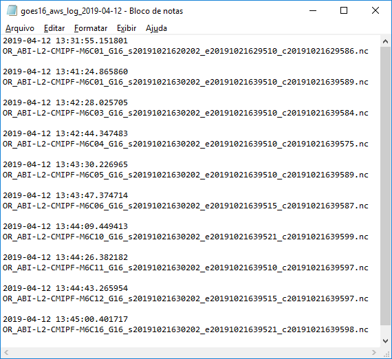
When executing the script, the output should be like this:

And the daily log will be created:

Containing all the files that have been downloaded:

If the script is called again, and the file is already on the log, you should see this message:

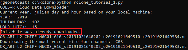
All right! Calling this script every “x” minutes will download the most recent GOES-16 Level 2 CMI (Full-Disk), for the selected channels! Just call the example script using the Linux “Cron” or the Windows “Task Scheduler”!

Simulating a “Cron” / “Task Scheduler” with Python

If you do not want to use the Cron or Task Scheduler, here’s a simple way to simulate a scheduler with Python:

import sched, time # Scheduler library
import os          # Miscellaneous operating system interfaces

# Interval in seconds
seconds = 60

# Call the function for the first time without the interval
print("\n")
print("------------- Calling Monitor Script --------------")
script = 'python rclone_tutorial_1.py'
os.system(script)
print("------------- Monitor Script Executed -------------")
print("Waiting for next call. The interval is", seconds, "seconds.")

# Scheduler function
s = sched.scheduler(time.time, time.sleep)

def call_monitor(sc):
print("\n")
print("------------- Calling Monitor Script --------------")
script = 'python rclone_tutorial_1.py'
os.system(script)
print("------------- Monitor Script Executed -------------")
print("Waiting for next call. The interval is", seconds, "seconds.")
s.enter(seconds, 1, call_monitor, (sc,))
# Keep calling the monitor

# Call the monitor
s.enter(seconds, 1, call_monitor, (s,))
s.run()

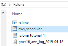
Let’s call it “aws_scheduler.py”:

When activating this script, the “rclone_tutorial_1.py” will be called every 60 seconds (you may change the interval on the “seconds” variable).

Here is an example of output when calling the “aws_scheduler.py” script:

And that’s it for Part I! Stay tuned for news!