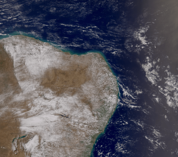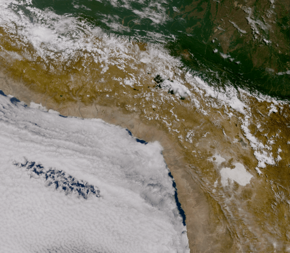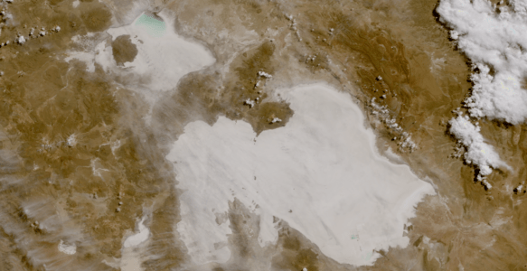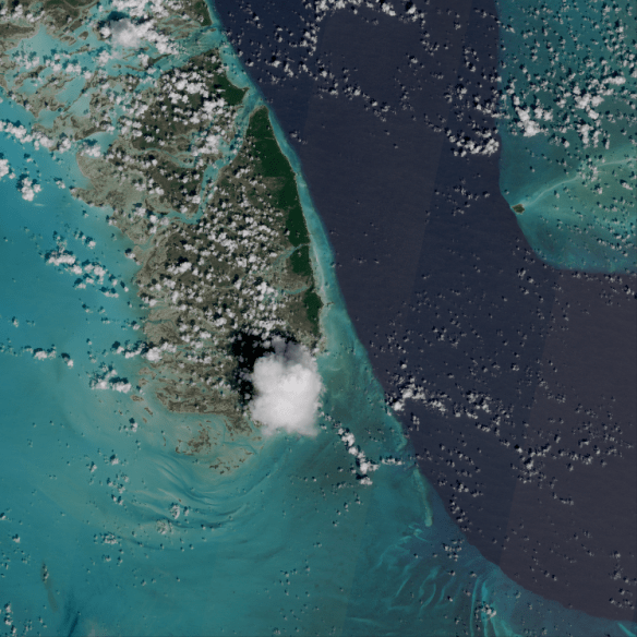
South Andros Island, Bahamas (09-25-2018, 15:55 UTC), shown by Sentinel-2 MSI (10 m resolution), processed with Python (Satpy). Data downloaded from the Copernicus Open Access Hub.
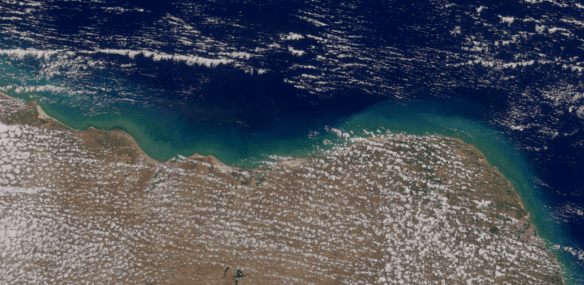
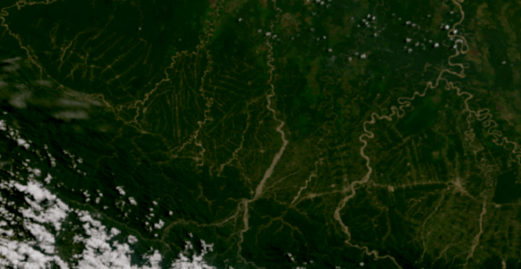
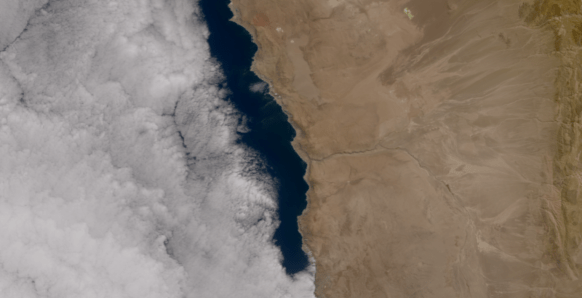
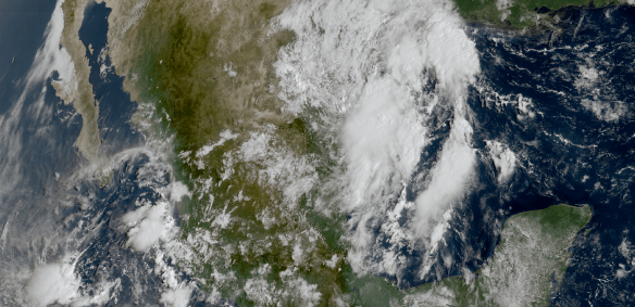
Below, some zooming in the image above!


As a follow up to the previous Blog post, where we shown how to process Sentinel-3 OLCI data, let’s see how to process Sentinel-2 MSI Data with Python. The process is very similar. Let’s see an example:
ACCESSING SENTINEL-2 DATA USING THE COPERNICUS OPEN ACCESS HUB
Access the Copernicus Open Access Hub at the following link:
scihub.copernicus.eu/dhus/

Create an account by clicking at the “Sign up” link on the LOGIN menu.
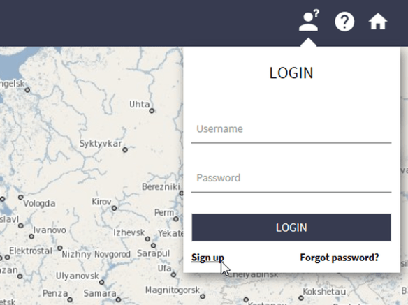


Awesome!
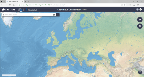
After creating an account, as it happened in the CODA from the previous Blog Post, navigate to the region of interest. In this example, Bahamas.
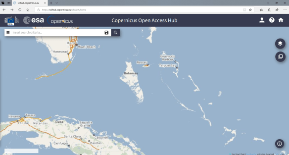
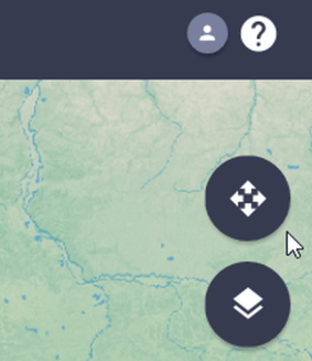
Now click on the following icon to select your region of interest:

And select the area:
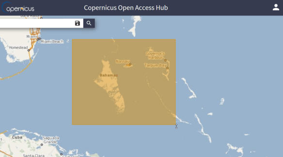
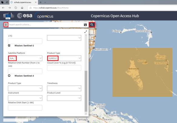
Expand the “Insert Search Criteria” menu. Under “Mission: Sentinel-2”, in “Satellite Platform” select “S2A_*”, in “Product Type”, choose “S2MSI1C”. Click at the magnifier icon to search for data over the select region.
You should see the available passes for that region:
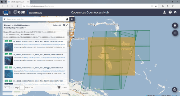
Let’s select this one:

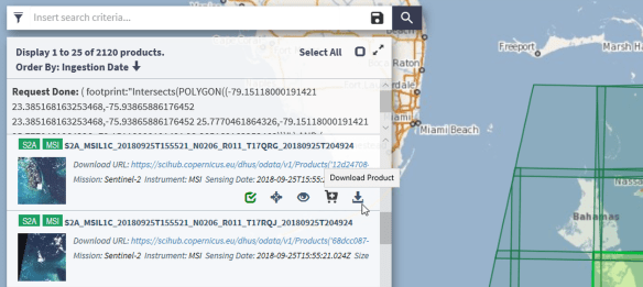
Click at the following icon to download the L1 data:
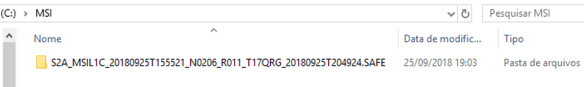
After the download, extract the data in the directory of you preference. In this example, we extracted it at C:\MSI
PROCESSING THE SENTINEL-2 DATA WITH SATPY
You should be familiar with Anaconda if you followed the GOES-16 and Python tutorials from this blog. Let’s make a quick overview.
Download the Anaconda Distribution from the following link:
After installing it, execute the Anaconda Prompt as an Admin:

Install SatPy in a new env using Anaconda and execute the Spyder IDE. Here are the commands we used:
conda create --name satellite
activate satellite

conda install -c conda-forge satpy
conda install -c conda-forge matplotlib
conda install -c conda-forge Pillow
conda install -c conda-forge pyorbital
conda install -c sunpy glymur
Use the following script to generate the True Color composite from that pass:
from satpy.scene import Scene
from satpy import find_files_and_readers
from datetime import datetime

files = find_files_and_readers(base_dir="C:\\MSI",
                               reader='safe_msi')

scn = Scene(filenames=files)
scn.load(['true_color'])
scn.save_dataset('true_color', filename='true_color_S2_gnc_tutorial'+'.png')
IMPORTANT NOTE: Given the high resolution of this image (10 m), this will require a good amount of RAM! And will generate a huge image (almost 200 MB).
And that’s it! This is what we get plotting this dataset!

Beautiful!
You can do many things using the features provided by Python / Satpy, like reprojection, exporting to other formats, overlaying maps and many other things!
You. Can. Do. Anything. With. Python.