Derived Motion Winds: A Python Script

DMWF_SAOPAULO_GNCA.png

Derived Motion Winds (Band 14) over the  Brazilian Southeast – Plot made with Python

DMW GNC-A Plot.gif

Derived Motion Winds (Band 14), animation made with Python

Hi GEONETCasters!

Lots of new Python examples for GNC-A products lately! 😆

Today we’ll show you how to manipulate the GOES-16 Derived Motion Winds baseline products that have been broadcasted through GNC-A since the beginning of March, as seen on this blog post.

DMWF_Ocean_GNCA

“I see wind vectors.” “How often do you see them?” “All the time.” 😯

The GOES-16 Derived Motion Winds NetCDF’s are received in the following folders:

DMW Folders GNC-A

  • GOES-R-Level-2-Products/DMWF-C02  (Winds Derived from ABI Band 02)
  • GOES-R-Level-2-Products/DMWF-C07  (Winds Derived from ABI Band 07)
  • GOES-R-Level-2-Products/DMWF-C08  (Winds Derived from ABI Band 08)
  • GOES-R-Level-2-Products/DMWF-C09  (Winds Derived from ABI Band 09)
  • GOES-R-Level-2-Products/DMWF-C10  (Winds Derived from ABI Band 10)
  • GOES-R-Level-2-Products/DMWF-C14  (Winds Derived from ABI Band 14)
  • GOES-R-Level-2-Products/DMWVF-C08 (Clear Sky Winds Derived from ABI Band 08)

Please find below some other examples:

DMWF_USA_GNCA

Derived Motion Winds (Band 14) over USA – Plot made with Python

DMWF_B08_GNCA

Derived Motion Winds (Band 08) over South America – Plot made with Python

DMWF_BRAZIL_GNCA

Derived Motion Winds (Band 14) over South America – Plot made with Python

DMWF_FULL_GNCA

GNC_Script_Download.png

Please download the script used to create these plots at this link.

Stay tuned for news! The GLM data will be added soon!

GNC_GOES-r.png

30,000 GEONETviews!

Blog Views 30000.png

GNC-A Blog readers by location

In the last week the GNC-A Blog reached 30000 views from more than 110 countries! Thank you to all our readers!

The most viewed pages this year are the following:

Blog Views 30000 2The top 10 visitor countries are:

  • 1 – Brazil
  • 2 – USA
  • 3 – Peru
  • 4 – Canada
  • 5 – Mexico
  • 6 – Germany
  • 7 – Colombia
  • 8 – Argentina
  • 9 – Cuba
  • 10 – Ecuador

GNC-A Station Monitoring With Zabbix

IPMet Bauru, one of the 32 Brazilian GNC-A users, kindly shared some screenshots of how they are monitoring their GNC-A station with Zabbix,  the  free and open source monitoring software for networks and applications. Zabbix was designed to monitor and track the status of various network services, servers, and other network hardware.

IMG-20180321-WA0014

The graph above shows four lines (from top to bottom):

  • Signal to Noise Ratio (dB)
  • “Trigger” Threshold: Satellite Signal Lost (SNR < 10 dB)
  • Bit Error Rate
  • Signal Strenght (dBm)

Note: This Blog post shows a script to extract these values from the NOVRA S300D Receiver.

When the first line, the Signal to Noise Ratio, goes below the “Trigger” level, the “Trigger” is activated (sending a notification e-mail for example).

The interface also monitors the network traffic:

IMG-20180322-WA0003

Please notice that the limit is 12 Mbps, the current GNC-A capacity.

Also, there’s a very nice scheme showing a summary of the status:

IMG-20180322-WA0002

An SNR above 15 dB! Wow! Can you get an SNR like this???

Very nice! The image below shows the station from IPMet:

IMG-20160830-WA0005b

IPMet also followed the Python Tutorial from this Blog and they are generating very nice plots using GOES-16 NetCDF’s:

IPMET GIF.gif

Thanks IPMet!

Day / Night Band: A Python Script

201803200449237

Beautiful Plot of the Day / Night Band made with Python, from March 20th 2018, 04:46 – 04:49 UTC

CIRA_RAMMB_Geocolor

Ever wondered from where the nigh lights on the amazing Geocolor RGB is obtained? Credits: RAMMB/CIRA SLIDER

GEONETCasters,

As seen on this  Blog post, you may find the Day / Night Band NetCDF’s inside the JPSS/BANDS/DNB GNC-A Folder:

Day night Band.png

Below, an animation showing the DNB over Brazil:

DayNightBandBrazil

Please find below an example script to manipulate these NetCDF’s (note: the interpolation to create the Georeference should be improved):

#########################################
# LICENSE
#Copyright (C) 2018 - INPE - NATIONAL INSTITUTE FOR SPACE RESEARCH
#This program is free software: you can redistribute it and/or modify it under the terms of the GNU General Public License as published by the Free Software Foundation, either version 3 of the License, or (at your option) any later version.
#This program is distributed in the hope that it will be useful, but WITHOUT ANY WARRANTY; without even the implied warranty of MERCHANTABILITY or FITNESS FOR A PARTICULAR PURPOSE. See the GNU General Public License for more details.
#You should have received a copy of the GNU General Public License along with this program. If not, see http://www.gnu.org/licenses/.
#########################################

# Required libraries ==================================================================================
import matplotlib.pyplot as plt # Import the Matplotlib package
import numpy as np # Import the Numpy package
from matplotlib.colors import LinearSegmentedColormap # Linear interpolation for color maps
from netCDF4 import Dataset # Import the NetCDF Python interface
import pyresample as pr
from pyresample import geometry
from pyresample.kd_tree import resample_nearest
import glob
from cpt_convert import loadCPT # Import the CPT convert function
import time as t
# You need to install the pyresample package!
# conda install -c conda-forge pyresample
#======================================================================================================
dirname = 'E:\\VLAB\\Python\\NPP Samples\\Sequence-DNB-19032017\\'
# Get all DNB files in the directory
DNB_images = []
for filename in sorted(glob.glob(dirname+'/VIIRS_NCC_EDR_npp*.nc')):
DNB_images.append(filename)

# Get all GEO files in the directory
DNB_geo = []
for filename in sorted(glob.glob(dirname+'/VIIRS_NCC_EDR_GEO*.nc')):
DNB_geo.append(filename)

# Convert user lat lons to bounding box with pyproj
import pyproj
prj = pyproj.Proj('+proj=eqc')
# The extent below only works with the Equidistant Projection
#extent = [-104, 8, -67, 31]
#extent = [-170.79949951171875, -81.32820129394531, -8.200499534606934, 81.32820129394531]
extent = [-80.0, -37.0, -30.0, 8.0]
lon_bbox = (extent[0], extent[2])
lat_bbox = (extent[1], extent[3])
x, y = prj(lon_bbox, lat_bbox)

# Final image size (you have to play with these to get the maximum res)
x_size = 3712 #464 #928 #3712 #7424
y_size = 3712 #464 #928 #3712 #7424

# Define the type of plot (satellite projection or rectangular, you have to choose only one)
#area_def = geometry.AreaDefinition('Orthographic', 'Ortho Globe', 'Orthographic', {'a': '6370998.0', 'units': 'm', 'lat_0': '0','lon_0': '-75', 'proj': 'ortho'}, x_size, y_size, [-6370998.0, -6370998.0, 6370998.0, 6370998.0])
area_def = geometry.AreaDefinition('Equidistant Cylindrical ', 'Plate Carree world map', 'Equidistant Cylindrical ', {'proj': 'eqc'}, x_size, y_size, [x[0], y[0], x[1], y[1]])

print("Plotting the Background")
start = t.time()

# Define the final image resolution (fixed value in this example. this may be changed to get maximum res)
DPI = 150
ax = plt.figure(figsize=(2000/float(DPI), 2000/float(DPI)), frameon=False, dpi=DPI)
ax = plt.axis('off')

# Create a basemap based on the area definition
bmap = pr.plot.area_def2basemap(area_def, resolution='i')

# Add the brazilian states shapefile
bmap.readshapefile('E:\\VLAB\\Python\\Shapefiles\\estados_2010','estados_2010',linewidth=0.50,color='gray')
# Add the countries shapefile
bmap.readshapefile('E:\\VLAB\Python\\Shapefiles\\ne_10m_admin_0_countries','ne_10m_admin_0_countries',linewidth=0.50,color='black')
# Add the continents shapefile
bmap.readshapefile('E:\\VLAB\\Python\\Shapefiles\\continent','continent',linewidth=2.00,color='black')

# Add a background
bmap.shadedrelief()

# Add parallels and meridians
bmap.drawparallels(np.arange(-90.0, 90.0, 10.0), linewidth=0.2, dashes=[4, 4], color='cyan')
bmap.drawmeridians(np.arange(0.0, 360.0, 10.0), linewidth=0.2, dashes=[4, 4], color='cyan')

print("Backgound Plot finished.")
print ('Time:', t.time() - start, 'seconds')

lons_interp = np.zeros((771,4121))
lats_interp = np.zeros((771,4121))

# Start the plot loop with the files in the directory (you have to insert the index range you want)
for x in range (5,6):
#for x in (i for j in (range(19, 27), range(41, 47)) for i in j):
# Get the image
path = DNB_images[x]

# Get the start of scan from the file name
Start = (path[path.find("_s")+2:path.find("_e")])

# Seek for a GEO file in the directory
matching = [s for s in DNB_geo if Start in s]

# If the GEO file is not found, exit the loop
if not matching:
print("GEO File Not Found! Exiting Loop.")
break
else: # If the GEO file is found, continue
print("GEO File OK!")
matching = matching[0].replace("\\\\", "\\")
index = DNB_geo.index(matching)
path2 = DNB_geo[index]

print("Processing file " + Start)
start = t.time()

# Open the file using the NetCDF4 library
nc = Dataset(path)
nc2 = Dataset(path2)

# Get the lats and lons from the GEO file
lats = nc2.variables['Latitude@VIIRS-NCC-EDR-GEO'][:]
lons = nc2.variables['Longitude@VIIRS-NCC-EDR-GEO'][:]

# Disable the auto scale (for some reason the automatic scale is giving errors)
nc.set_auto_maskandscale(False)
data = nc.variables['Albedo@VIIRS-NCC-EDR'][:]
scale = nc.variables['Albedo@VIIRS-NCC-EDR'].scale_factor
offset = nc.variables['Albedo@VIIRS-NCC-EDR'].add_offset
# Apply the scale and offset
data = (data * scale) + offset

# Get rid of the bad values
data[data >= 380] = np.nan

# We have a condensed GEO file (only 3 columns). We need to interpolate.
# This is using linear interpolation only! We are working to make this
# more efficient.
lons_interp = np.zeros((771,4121))
lats_interp = np.zeros((771,4121))

factor = 1.013
for x in range (0,771):
if np.isnan(lons[x,0]) == False:
lons_interp[x,0:1030] = (np.array([np.linspace(lons[x,0],(lons[x,0]+lons[x,1])/2, 1030)]))
lons_interp[x,1031:2061] = (np.array([np.linspace((lons[x,0]+lons[x,1])/2,lons[x,1], 1030)]))
lons_interp[x,2062:3092] = (np.array([np.linspace(lons[x,1],(lons[x,1]+lons[x,2])/2, 1030)]))
lons_interp[x,3091:4121] = (np.array([np.linspace((lons[x,1]+lons[x,2])/2,lons[x,2], 1030)]))
if np.isnan(lats[x,0]) == False:
lats_interp[x,0:1030] = (np.array([np.linspace(lats[x,0],((lats[x,0]+lats[x,1])/2)*factor, 1030)]))
lats_interp[x,1031:2061] = (np.array([np.linspace(((lats[x,0]+lats[x,1])/2)*factor,lats[x,1], 1030)]))
lats_interp[x,2062:3092] = (np.array([np.linspace(lats[x,1],((lats[x,1]+lats[x,2])/2)*factor, 1030)]))
lats_interp[x,3091:4121] = (np.array([np.linspace(((lats[x,1]+lats[x,2])/2)*factor,lats[x,2], 1030)]))

# Define the swath
swath_def = pr.geometry.SwathDefinition(lons_interp, lats_interp)

# Get a result with the pyresample magic
result = resample_nearest(swath_def, data, area_def, radius_of_influence=2000, fill_value=None)

# Plot the final image
col = bmap.imshow(result, origin='upper', vmin=-1, vmax=7, cmap='gray')

# Save the result
ax = plt.savefig('E:\\VLAB\\Python\\NPP Samples\\Output\\' + Start, dpi=DPI, bbox_inches='tight', pad_inches=0)
plt.close()
print("Processing finished.")
print ('Time:', t.time() - start, 'seconds')

print("Program finished.")

Please find below other blog posts about JPSS and GNC-A:

JPSS.png

New Operational GNC-A Station: SMN-ARGENTINA (Station n° 78!)

We have a new GNC-A operational station! It was installed at the SMN, the National Weather Service of Argentina. This is the second GNC-A station in Argentina, along with CONAE. Two more stations are planned!

The SMN’s GNC-A antenna is shown at the picture below:

Argentina - SMN.png

GEONETCast-Americas and the “Do It Yourself” way to receive environmental data in near real time

And below, the KenCast software ingesting GOES-16 files:

IMG-20180322-WA0036

GOES-16 files being received at SMN-Argentina

The station was used to receive the EUMETCast-Americas broadcast and now it has been converted to GNC-A. This is part of the setup they are using:

Antenna:

  • Manufacturer: Sami Dish (USA)
  • Model: Mesh

LNB:

  • Manufacturer: Yokowo (Japan)
  • Model: YOM-4307

DVB-S Receiver:

Argentina - SMN 2.png

Great job SMN-Argentina team! Thanks Diana, Maxi and Estela for sharing the experience!

GNC-SMN.png

Welcome to the community SMN!

Blended TPW and TPW Anomaly Products: A Python Script

BTPW_Animation.gif

Blended TPW animation made with Python. The data is derived from several data sources, including the Special Sensor Microwave / Imager (SSM/I) passes from the Defense Meteorological Satellites Program (DMSP), the Advanced Microwave Sounding Unit (AMSU) from Polar Operational Environmental Satellites (POES), and information from Global Positional Satellite (GPS) meteorological data.

BTPW-PCT_Animation.gif

TPW Anomaly animation made with Python. The TPW anomaly assists forecasters to answer the question, “How unusual is the moisture field?”. Very high percentage values (200% or more) indicate a strong flooding potential or a possible severe weather indicator, while low values indicate potential fire hazards.

Hi GEONETCasters,

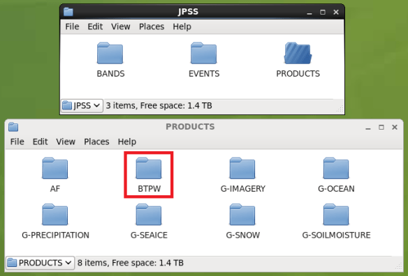
As seen on this and this Blog posts, you may find hourly Blended Total Precipitable Water and Total Precipitable Water Anomaly Products inside the JPSS/PRODUCTS/BTPW GNC-A Folder.

JPSS-BTPW-FOLDER.png

The file naming convention for these files are:

  • NPR.COMP.TPW.Syydddhhmm.Eyydddhhmm.Thhmmss.he4
  • NPR.COMP.PCT.Syydddhhmm.Eyydddhhmm.Thhmmss.he4

Where:

yy = year
jjj = julian day
hh = hour
mm = minutes
ss = seconds

D = day
S = start
E = end
T = time

These represent the year and julian day of the data covered, the start (“S”) and end (“E”) time in hour and minutes for which the data of the image covers, and the creation time (“T”) of the image in julian day, hour, and minutes.

Please find below an example Python script to manipulate these products.

Within the script you may also choose the region you want to plot. In the examples below the Brazilian region was chosen (BTPW on the left and TPW anomaly on the right).

In order to run the script, you need to install the pyhdf library. Here’s the conda command to download it:

conda install -c conda-forge pyhdf 

Also, you must have the following text files referenced in the script (click to download):

###############################################################################
# LICENSE
#Copyright (C) 2018 - INPE - NATIONAL INSTITUTE FOR SPACE RESEARCH
#This program is free software: you can redistribute it and/or modify it under the terms of the GNU General Public License as published by the Free Software Foundation, either version 3 of the License, or (at your option) any later version.
#This program is distributed in the hope that it will be useful, but WITHOUT ANY WARRANTY; without even the implied warranty of MERCHANTABILITY or FITNESS FOR A PARTICULAR PURPOSE. See the GNU General Public License for more details.
#You should have received a copy of the GNU General Public License along with this program. If not, see http://www.gnu.org/licenses/.
###############################################################################
# Required libraries ==========================================================
import matplotlib.pyplot as plt # Import the Matplotlib package
from mpl_toolkits.basemap import Basemap # Import the Basemap toolkit
import numpy as np # Import the Numpy package
import datetime # Library to convert julian day to dd-mm-yyyy
# conda install -c conda-forge pyhdf
from pyhdf.SD import SD, SDC
# =============================================================================
# Reading the file:
path = 'E:\\VLAB\\Python\\TPW Samples\\NPR.COMP.TPW.S180310337.E180311226.T134745.he4'
file = SD(path, SDC.READ)
#print (file.info())
datasets_dic = file.datasets()
#for idx,sds in enumerate(datasets_dic.keys()):
#print (idx,sds)
# Detecting if is BTPW or PCT:
product = (path[path.find("COMP.")+5:path.find(".S")])
if (product == "TPW"):
sds_obj = file.select('TPW_Mean') # select sds
product = "BTPW"
elif (product == "PCT"):
sds_obj = file.select('TPW_Percent') # select sds
product = "BTPW_PCT"

data = sds_obj.get() # get sds data
# The pixels without values are set with "-1". You may replace it with a nan if you want
#data[data == -1] = np.nan
# =============================================================================
# Reading Longitudes ==========================================================
with open('E:\\VLAB\\Python\\TPW Samples\\A_BTPW_Longitude.txt') as f:
longitudes = f.readlines()
num_linhas = len(longitudes)

lon = []

for x in range (2,num_linhas):
valores = longitudes[x].strip()
valores = valores.split()
lon.append(float(valores[2]))

f.close()

lons = np.asarray(lon)

# Reading Latitudes ===========================================================
with open('E:\\VLAB\\Python\\TPW Samples\\A_BTPW_Latitude.txt') as f:
latitudes = f.readlines()

num_linhas = len(latitudes)

lat = []

for x in range (2,num_linhas):
valores = latitudes[x].strip()
valores = valores.split()
lat.append(float(valores[2]))

f.close()

lats = np.asarray(lat)
# =============================================================================
# Defining the plot extent:

# GOES-East
#extent = [-156.29949951171875, -60.0, 6.299499988555908, 60.0]

# South America
#extent = [-90.0, -60.0, -30.0, 15.0]

# Full Extent
extent = [-180, -71.24783, 180, 71.24783]

# Latitude lower and upper index:
latli = np.argmin( np.abs( lats - extent[1] ) )
latui = np.argmin( np.abs( lats - extent[3] ) )

if (extent[2] > 20):
# Longitude lower and upper index:
lonli = np.argmin( np.abs( lons - extent[0] ) )
lonui = np.argmin( np.abs( extent[2] - lons ) )
data1 = data[latui:latli , lonli:2499]
data2 = data[latui:latli , 0:lonui]
data = np.hstack((data1, data2))
else:
# Longitude lower and upper index:
lonli = np.argmin( np.abs( lons - extent[0] ) )
lonui = np.argmin( np.abs( lons - extent[2] ) )
data = data[latui:latli , lonli:lonui]

# Define the size of the saved picture=========================================
DPI = 150
fig = plt.figure(figsize=(data.shape[1]/float(DPI), data.shape[0]/float(DPI)), frameon=False, dpi=DPI)
ax = plt.Axes(fig, [0., 0., 1., 1.])
ax.set_axis_off()
fig.add_axes(ax)
ax = plt.axis('off')
#==============================================================================

# Create the Basemap
bmap = Basemap(projection='merc',llcrnrlon=extent[0], llcrnrlat=extent[1],urcrnrlon=extent[2], urcrnrlat=extent[3], resolution='l')

# Draw parallels and meridians
bmap.drawparallels(np.arange(-90.0, 90.0, 5.0), labels=[False,False,False,False], dashes=[5, 5], linewidth=0.2, fontsize=8, color='grey')
bmap.drawmeridians(np.arange(0.0, 360.0, 5.0), labels=[False,False,False,False], dashes=[5, 5], linewidth=0.2, fontsize=8, color='grey')

# Add the brazilian states shapefile
bmap.readshapefile('E:\\VLAB\\Python\\Shapefiles\\estados_2010','estados_2010',linewidth=0.30,color='gray')
# Add the countries shapefile
bmap.readshapefile('E:\\VLAB\Python\\Shapefiles\\ne_10m_admin_0_countries','ne_10m_admin_0_countries',linewidth=0.50,color='black')
# Add the continents shapefile
bmap.readshapefile('E:\\VLAB\\Python\\Shapefiles\\continent','continent',linewidth=1.00,color='black')

# Show image
if (product == "BTPW"):
bmap.imshow(data, origin='upper', cmap='rainbow', vmin = 0, vmax = 70)
elif (product == "BTPW_PCT"):
bmap.imshow(data, origin='upper', cmap='rainbow', vmin = 0, vmax = 300)

# Getting information from the file name ======================================
# Search for the Scan start in the file name
Start = (path[path.find(".S")+2:path.find(".E")])

# Converting from julian day to dd-mm-yyyy
year = int('20' + (Start[0:2]))
dayjulian = int(Start[2:5]) - 1 # Subtract 1 because the year starts at "0"
dayconventional = datetime.datetime(year,1,1) + datetime.timedelta(dayjulian) # Convert from julian to conventional
#print (dayconventional)
date = dayconventional.strftime('%d%m%Y') # Format the date according to the strftime directives
date_formatted = dayconventional.strftime('%d-%m-%Y')

# Search for time in the filename
Time = path[-10:]
Hour = Time [0:2]
Minutes = Time [2:4]
Seconds = Time [4:6]

time = Hour + ":" + Minutes + ":" + Seconds + " UTC"

# Colorbar ====================================================================
# Plot a colorbar
if (product == "BTPW"):
cb = bmap.colorbar(location='bottom', size = '2%', ticks=[5,10,15,20,25,30,35,40,45,50,55,60,65], pad = '-2.0%')
elif (product == "BTPW_PCT"):
cb = bmap.colorbar(location='bottom', size = '2%', ticks=[25,50,75,100,125,150,175,200,225,250,275], pad = '-2.0%')
# Remove the colorbar outline
cb.outline.set_visible(False)
# Remove the colorbar ticks
cb.ax.tick_params(width = 0)
# Put the colobar labels inside the colorbar
cb.ax.xaxis.set_tick_params(pad = -14)
# Change the color and size of the colorbar labels
cb.ax.tick_params(axis='x', colors='black', labelsize=10)
# =============================================================================
# Legend ======================================================================
if (product == "BTPW"):
cb.set_label('GNC-A Blog: Blended Total Precipitable Water [mm] ' + date_formatted + " " + time, color='white', size = 15)
elif (product == "BTPW_PCT"):
cb.set_label('GNC-A Blog: Total Precipitable Water Anomaly [%] ' + date_formatted + " " + time, color='white', size = 15)
cb.ax.xaxis.set_label_position('top')
cb.ax.xaxis.set_label_coords(0.245, 1.5)
# =============================================================================
# Add logos / images to the plot ==============================================
logo_GNC = plt.imread('E:\\VLAB\\Python\\Logos\\GNC Logo - White.png')
logo_INPE = plt.imread('E:\\VLAB\\Python\\Logos\\INPE Logo.png')
logo_NOAA = plt.imread('E:\\VLAB\\Python\\Logos\\NOAA Logo.png')
logo_JPSS = plt.imread('E:\\VLAB\\Python\\Logos\\JPSS Logo.png')
plt.figimage(logo_GNC, 10, 80, zorder=3, alpha = 1, origin = 'upper')
plt.figimage(logo_INPE, 390, 80, zorder=3, alpha = 1, origin = 'upper')
plt.figimage(logo_NOAA, 490, 80, zorder=3, alpha = 1, origin = 'upper')
plt.figimage(logo_JPSS, 590, 80, zorder=3, alpha = 1, origin = 'upper')
# =============================================================================
# =============================================================================

# Save the result
plt.savefig('E:\\VLAB\\Python\\Output\\JPSS_' + product + '_' + date + Hour + Minutes + Seconds + '.png', dpi=DPI, pad_inches=0)
plt.close()

For more details about the above files and what they contain, please visit the OSPO BTPW homepage http://www.ospo.noaa.gov/Products/bTPW/Overview.html, where you can find various kinds of information about the bTPW product and what it represents.

Please find below other blog posts about JPSS and GNC-A:

JPSS.png

First Tests With GOES-16 Level 2 Data And Python

Hi GEONETCasters,

The first Level 2 Baseline Products from GOES-16 have been added to the broadcast (Derived Motion Winds for now), as seen at this Blog post. More products will be added, as soon as they reach the “Provisional” maturity level. This will happen along the year, as seen on the image below (dates subject to change):

21.png

Meanwhile, we’re testing a Python script able to manipulate these products. Please find below some preliminary plots (Note: Most of these products are in Beta maturity!):

  • Cloud Top Height:

G16_ACHAF_HT_201802271400

  • Cloud Top Temperature:

G16_ACHTF_TEMP_201802220415

  • Clear Sky Masks:

G16_ACMF_BCM_201802271400

  • Cloud Top Phase:

G16_ACTPF_Phase_201802271400

  • Aerosol Optical Depth:

G16_AODF_AOD_201802271345

  •  Volcanic Ash (Air Mass Loading):

G16_VAAF_VAML_201802271345

  •  Volcanic Ash (Ash Cloud Height):

G16_VAAF_VAH_201802271345

  • Total Precipitable Water:

G16_TPWF_TPW_201802271400

  • Sea Surface (Skin) Temperature:

G16_SSTF_SST_201802271200

  • Rainfall Rate – Quantitative Prediction Estimate:

G16_RRQPEF_RRQPE_201802271400

  • Land Surface (Skin) Temperature:

G16_LSTF_LST_201802271300

  • Snow Cover:

G16_FSCF_FSC_201802271345

  • Fire-Hot Spot Characterization (Mask):

G16_FDCF_Mask_201802271400

  • Derived Stability Indices (Total Totals Index):

G16_DSIF_TT_201802271345

  • Derived Stability Indices (Showalter Index):

G16_DSIF_SI_201802271345

  • Derived Stability Indices (Lifted Index):

G16_DSIF_LI_201802271345

  • Derived Stability Indices (K-Index):

G16_DSIF_KI_201802271345

  • Derived Stability Indices (CAPE):

G16_DSIF_CAPE_201802271345

  • Cloud Particle Size:

G16_CPSF_PSD_201802220415

  • Cloud Optical Depth:

G16_CODF_COD_201802271345

Some products have not been added to the script yet (the derived motion winds for example). But they’re on the way.

All these plots were made using a single script and a single “remap.py” file. The idea is to have a single script to manipulate any GOES-16 files, including the channels.

Things are getting fun. Stay tuned for news.

New GOES-16 and JPSS Products Added To GNC-A

Dear GEONETCasters,

Today, the following products have been added to the GNC-A broadcast:

  • GOES-16 Derived Motion Winds (Bands 02, 07, 08, 09, 10 and 14)
  • Global Blended Total Precipitable Water
  • Suomi NPP Active Fires

The GOES-16 Derived Motion Winds NetCDF’s are received in the following folders:

GOES-R-Level-2-Products/DMWF-C02
GOES-R-Level-2-Products/DMWF-C07
GOES-R-Level-2-Products/DMWF-C08
GOES-R-Level-2-Products/DMWF-C09
GOES-R-Level-2-Products/DMWF-C10
GOES-R-Level-2-Products/DMWF-C14
GOES-R-Level-2-Products/DMWVF-C08

180129_goes16_infrared_winds_anim.gif

Low-Level Infrared-Cloud Drift Winds – UW-CIMMS/NESDIS

The hourly Global Blended Total Precipitable Water HDF’s are received in the following folder:

JPSS/PRODUCTS/BTPW

GLOBAL_TPW_20180308_12Z

The Active Fires TXT’s are received in the following folder:

JPSS/PRODUCTS/AF

This is an example of the Active Fire Product in it’s text format, with latitudes, longitudes, and other information:

Fire Text File.png

And here is an example of the information plotted in a map:

ActiveFiresNDE_20160318_lg.png

We’ll post how to manipulate these products in the near future.

GOES-16 GLM Data To Be Added Soon In GNC-A

GLM Example

GLM Flash Density over the last 5 minutes, plot made with Python

Dear GEONETCasters,

The Geostationary Lightning Mapper Flash Density Product (accumulated every 5 minutes) will be added to the GEONETCast-Americas broadcast soon!

For every ABI Full Disk NetCDF (15 minutes) you’ll receive three GLM NetCDF’s, each with the number of flashes detected over the last 5 minutes.

This will be the naming convention:

DENS_YYYYMMDDHHMN00.nc

Please download a sample at this link. You may download an ABI NetCDF for this time frame at this link.

It will be available at the “GOES-R-GLM-Products” folder in your GNC-A ingestion directory.

Each NetCDF contains an 8 x 8 km regular grid with all flashes detected in the last 5 minutes. The original frequency was 20 seconds. To make things easier for users, this 5 minute density was created.

If you’re already processing the GOES-16 files with Python, this is the only piece of code you’ll need to add to overlay the flashes with the ABI imagery:

# Processing the GLM file =====================================================
path_GLM = 'E:\\VLAB\\Python\\GLM Samples\\DENS_30003_20180213200500.nc'
dataglm=Dataset(path_GLM)

lats_file=dataglm.variables['lat'][:]
lons_file=dataglm.variables['lon'][:]
dens_file=dataglm.variables['dens'][:]

dens=dens_file[0,:,:]

lons, lats = np.meshgrid(lons_file,lats_file)
lonss, latss = bmap(lons,lats)

cs_a1 = bmap.pcolormesh(lonss,latss,dens,cmap='rainbow', vmin = 0, vmax = 30)
# GLM Processing Finished =====================================================

Let’s check how it looks when plotted with Python, overlayed with a GOES-16 image:

ABI + GLM.pngABI + GLM 2.png

Now with the ABI image enhanced:

ABI + GLM 3.png

Not so visible huh? Let’s increase the ABI image transparency:

ABI + GLM 5.png

Much better! You may play with the transparency of the ABI image changing the “alpha” parameter of the following command:

bmap.imshow(data, origin='upper', cmap=cpt_convert, vmin=-103, vmax=84, alpha = 0.4)

ABI + GLM 6.png

Another great addition to the GNC-A Product list!