This is the tenth part of the GOES-16 / Python tutorial series. You may find the other parts by clicking at the links below:

• Part 1: Extracting Values and Basic Plotting
• Part 2: Basemaps, Grids, Legend and Exporting the Result
• Part 3: Getting information from the file name and header
• Part 4: Adding a background, changing transparency and adding a land / sea mask
• Part 5: Adding Shapefiles and using CPT color tables
• Part 6: Reprojection, Subsecting, Resolution and Julian Day Conversion
• Part 7: Better Look, K to °C, Add Logos and Export to GeoTIFF
• Part 8: Reprojecting CONUS, Mesoscales and NetCDF’s in other domains
• Part 9: Full Resolution Plots and Removing Image Borders

In this part, we’ll learn:

• How to automate the generation of products

-THE PROBLEM-

We received several e-mails from Blog readers asking how to use the scripts shown in the other parts operationally.

As seen in the script from PART IX for example, in the “path” variable, we select a single GOES-16 NetCDF file:

# Load the Data
# Path to the GOES-16 image file
path = 'E:\\VLAB\\Python\\GOES-16 Samples\\OR_ABI-L2-CMIPF-M3C13_G16_s20180571300407_e20180571311185_c20180571311263.nc'

And in the end, we save a single PNG file:

# Save the result
plt.savefig('E:\\VLAB\\Python\\Output\\G16_C' + str(Band) + '_' + date_save + '_' + time_save + '.png', dpi=DPI, pad_inches=0)
plt.close()

The question is, how to generate products automatically using this script, processing different NetCDF’s arriving at your ingestion folder, without your intervention.

-THE HUGE PROBLEM-

There are LOTS of ways to do it, using lots of different programming languages and procedures. In this Blog post we’ll show a simple approach, using Python.

-ONE OF MANY SOLUTIONS-

Basically, we’ll  follow the procedure described on the flowchart below:

Before trying to follow the procedure above, let’s see some basic concepts:

1 – Calling a python script from terminal / command prompt:

Let’s suppose our script from the tutorial Part IX is called “process_goes-16.py”.

If we are using Linux, we just need to type “python” and the name of our script (“.py” file):

python /home/VLAB/Scripts/process_goes-16.py

… or, if you’re already on your script directory:

/home/VLAB/Scripts# python process_goes-16.py

If we are using Windows, and want to use the “python” command anywhere, first we have to add our “python.exe” dilrectory to the “Path” system variable. On Windows 10, go to “Control Panel” > “All Control Panel Items” > “System”, choose “Advanced system settings”, on the “Advanced” tab, choose “Environment Variables”. On “System Variables”, click on the “Path” variable and choose “Edit…”. Add the directory where you have your “python.exe”, as the example below:

Now we can use the “python” command anywhere:

However, if we take a look at our code from Part IX for example, we are specifying the GOES-16 file to process:

If you’re using Linux, we could have for example:

# Load the Data =======================================================================================
# Path to the GOES-16 image file
path = '//home//VLAB//GOES-16 Samples//OR_ABI-L2-CMIPF-M3C13_G16_s20180571300407_e20180571311185_c20180571311263.nc'

If you’re using Windows, we could have for example:

# Load the Data =======================================================================================
# Path to the GOES-16 image file
path = 'E:\\VLAB\\GOES-16 Samples\\OR_ABI-L2-CMIPF-M3C13_G16_s20180571300407_e20180571311185_c20180571311263.nc'

So, when you execute your script using python process_goes-16.py it will always execute that single image.

We want to process a different image everytime we call the script process_goes-16.py, and to do that, we need to pass the NetCDF file name as an argument, the second concept we’ll cover before trying the flowchart procedure.

2 – Passing arguments to your python script

There is more than a single way to do it. In this Blog post we’ll see how to do it using the python “sys” (system specific parameters and functions) module.

First of all, import the “sys” module in your code:

import sys # Import the "system specific parameters and functions" module

Then, we may retrieve the following within the code:

• Name of the script: sys.argv[0]
• Argument n° 1: sys.argv[1]
• Argument n° 2: sys.argv[2]
• Argument n° 3: sys.argv[3]
• Argument n° “x”: sys.argv[“x”]

and so on…

We can also retrieve:

• Number of arguments: len(sys.argv)
• The arguments names as strings: str(sys.argv)

So, let’s think on how this can be useful.

Supposing I would like to pass a NetCDF file to be processed to my script. If I use the following command:

/home/VLAB/Scripts# python process_goes-16.py "E:\\VLAB\\Python\\GOES-16 Samples\\OR_ABI-L2-CMIPF-M3C13_G16_s20180571300407_e20180571311185_c20180571311263.nc"

I would have the following in my code:

• sys.argv[0] = process_goes-16.py
• sys.argv[1] = “E:\\VLAB\\Python\\GOES-16 Samples\\OR_ABI-L2-CMIPF-M3C13_G16_s20180571300407_e20180571311185_c20180571311263.nc”

Then, in the “path” variable, I could use:

# Load the Data =======================================================================================
# Path to the GOES-16 image file
path = sys.argv[1]

Let’s suppose I would like to pass, apart from the file name, the desired resolution. I could use the following command:

/home/VLAB/Scripts# python process_goes-16.py "E:\\VLAB\\Python\\GOES-16 Samples\\OR_ABI-L2-CMIPF-M3C13_G16_s20180571300407_e20180571311185_c20180571311263.nc" 2

Then, I would have the following in my code:

• sys.argv[0] = process_goes-16.py
• sys.argv[1] = “E:\\VLAB\\Python\\GOES-16 Samples\\OR_ABI-L2-CMIPF-M3C13_G16_s20180571300407_e20180571311185_c20180571311263.nc”
• sys.argv[2] = 2

Then, in the “resolution” variable, I could use:

resolution = int(sys.argv[2])

And this is it. You may pass the arguments you want to your script (like, the extent, name of the resulting file, colors, etc)

3 – Creating a log file with the file names of the NetCDF’s you already processed

Another important aspect of our automation process is that we need to create a log file, containing the file names that we have already processed.

In the end of your script, we could use the following code:

# Save the result as a PNG
plt.savefig('E:\\VLAB\\Python\\Output\\G16_C' + str(Band) + '_' + date_save + '_' + time_save + '.png', dpi=DPI, pad_inches=0, transparent=True)
plt.close()

# Add to the log file (called "G16_Log.txt") the NetCDF file name that I just processed.
# If the file doesn't exists, it will create one.
with open('E:\\VLAB\\Python\\Output\\G16_Log.txt', 'a') as log:
 log.write(path.replace('\\\\', '\\') + '\n')
#======================================================================================================

This will create a log file called “G16_Log.txt”. After each script execution a new line will be created with the file name that was just processed.

4 – Generate images without having a window appear,

Remember that each time we execute our scripts a plot window appears with the result preview? We will automate the PNG’s generation, so we don’t need that anymore. Also, this could result the error “Invalid Display Variable” when calling the scripts via the Linux Cron. Let’s disable this previsualization, adding the following to our code, before anything else in the code:

import matplotlib
matplotlib.use('Agg') # use a non-interactive backend

All right, we know the basics in order to begin implementing our flowchart. Let’s see how to do it, step by step:

A – Creating the “monitor” script

Now we need a script to monitor a given folder (e.g. your GNC-A folder for GOES-16 Band 13, for example). Let’s call this script “monitor.py”.

VERY IMPORTANT: This Blog post will be a “living blog post”. The example monitor script below is very very basic. We will post more advanced ones in the future. If you have any suggestions, feel free to use the comments section!

This script will perform the following tasks:

• Put all file names on the directory in a Python list
• Put all file names on the log created in Step 3 in a Python list
• Compare the directory list with the file list
• For each file in the directory that is not on the log, execute the script process_goes-16.py, passing the file as the argument

Please find below a suggestion for the monitoring script:

import glob # Unix style pathname pattern expansion
import os # Miscellaneous operating system interfaces

# Directory where you have the GOES-16 Files
dirname = 'E:\\VLAB\\Python\\GOES-16 Samples\\'

# Put all file names on the directory in a list
G16_images = []
for filename in sorted(glob.glob(dirname+'OR_ABI-L2-CMIPF-M3C13_G16*.nc')):
 G16_images.append(filename)

# If the log file doesn't exist yet, create one
file = open('E:\\VLAB\\Python\\Output\\G16_Log.txt', 'a')
file.close()

# Put all file names on the log in a list
log = []
with open('E:\\VLAB\\Python\\Output\\G16_Log.txt') as f:
 log = f.readlines()

# Remove the line feed
log = [x.strip() for x in log]

# Compare the directory list with the file list
# Loop through all files in the directory
for x in G16_images:
 # If a file is not on the log, process it
 if x not in log:
  os.system("python " + "\"E:\\VLAB\\Python\\Scripts\\process_goes-16.py\"" + " " + "\"" + x.replace('\\','\\\\') + "\"")

Note: If you’re using linux, you should specify in the “os.system” command instruction the full path for your python interface. If you don’t know it, you may use the python –version command to check which version you’re using and the python -v command to check the full path.

for x in G16_images:
 # If a file is not on the log, process it
 if x not in log:
 os.system("//root//anaconda3//bin//python " + "\"//home//VLAB//Scripts//process_goes-16.py\"" + " " + "\"" + x.replace('\\','\\\\') + "\"")

Now we have everything we need: A log file, an script that monitor a folder and a script that generate the plots. We just need one more thing, the periodic execution of the monitor script.

B – Put your script in the Linux Cron or in the Windows Task Scheduler 

If you’re using Linux, the process is pretty straightforward:

Edit your crontab using the crontab -e command. Choose your editor of preference. If you want to edit it with GEDIT, use the following command:

env EDITOR=gedit crontab -e

The GOES-16 images are received every 15 minutes, so let’s put the monitor.py script to run every 15 minutes. You also have to use the full path for your python interface.

*/15 * * * * /root/anaconda3/bin/python /home/VLAB/Scripts/monitor.py > /home/VLAB/Output/python.log 2>&1

Note: Any errors will be reported on the python.log file. Check this if you do not get your files processed after a cron activation.

If you’re using Windows, the process is a little bit longer:

Create a “.bat” file with the following command (adapt it according to your monitor.py script location):

python “E:\\VLAB\\Python\\Scripts\\monitor.py”

Note: To create a “.bat” file, just open a new Notepad document and save it with the “.bat” extension.

This is what this will look like:

Access the Windows Task Scheduler. In Windows 10, it is located at “Control Panel” > “Administrative Tools” > “Task Scheduler”.

In the upper menu, go to “Action” > “Create Basic Task…” or just click at “Create Basic Task…” on the right side of the window.

Follow the instructions below:

• In “Name”, put “Process GOES-16” for example. Click “Next”.
• In “When do you want the task to start?”, choose “Daily”. Click “Next”.
• In “Start”, change the time to “00:00:00” of the current day. Click “Next”.
• In “Action”, choose “Start a program”. Click “Next”.
• In “Program/script:” choose the “monitor.bat” we just created. Click “Next”.

• In the next window, where it shows the task summary, click “Finish”.

The task was created. Now we have to change it’s properties so it is executed every 15 minutes.

Back to the Task Scheduler main window, in “Active Tasks”, find the “Process GOES-16” task and double click it:

At the right side, chosse “Properties”, go to the “Triggers” tab, click on the Trigger and choose “Edit”.

Enable the “Repeat task every:” option, choosing “15 minutes”.

In the “for a duration of:” option, choose “Indefinitely”. Click “OK” and “OK” again.

This is what you should have in the “Active Tasks”:

For the “Process GOES-16” task, the “Trigger” message will say “At 00:00 every day – After treiggered, repeat every 15 minutes indefinitely”.

-FINISHED!-

And this is it! In both Windows and Linux, the monitor.py script will be called every 15 minutes and the process_goes-16.py script will be activated for every unprocessed GOES-16 NetCDF file on the target directory.

IMPORTANT: Please be aware that, when running the monitor script for the first time, it may take a while to process all the files, depending on the number of files you have in your directory. We suggest running this once before adding it to cron / task scheduler.

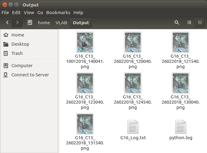
The image below shows a sequence on PNG’s created automatically:

And the same for Linux:

Stay tuned for the next tutorial part, where we’ll show how to create georeference files for your processed images, so they can be opened with SIGMACast (and other software also!)

This is the ninth part of the GOES-16 / Python tutorial series. You may find the other parts by clicking at the links below:

• Part 1: Extracting Values and Basic Plotting
• Part 2: Basemaps, Grids, Legend and Exporting the Result
• Part 3: Getting information from the file name and header
• Part 4: Adding a background, changing transparency and adding a land / sea mask
• Part 5: Adding Shapefiles and using CPT color tables
• Part 6: Reprojection, Subsecting, Resolution and Julian Day Conversion
• Part 7: Better Look, K to °C, Add Logos and Export to GeoTIFF
• Part 8: Reprojecting CONUS, Mesoscales and NetCDF’s in other domains

IMPORTANT: Since the last tutorial part (from Oct 10 2017), GOES-16 changed it’s position from 89.5 W to 75 W as the operational GOES East. We should use a new remap .py file, available for download at this link.

In this part, we’ll learn:

• How to make REALLY full resolution plots, independent of the selected extent (making some corrections on the previous code) and remove the saved image border completely.

-THE PROBLEM-

We received some e-mails from Blog readers reporting that the resolution of the generated image, depending on the image extent, wasn’t faithfull to the full NetCDF resolution, even if they choose the maximum resolution on the “resolution” variable.

Let’s check that.

Download the image from this link (channel 13 from Feb 26 2018, 13:00 UTC), and plot it using the script from Part VIII, with full extent:

extent = [min_lon, min_lat, max_lon, max_lat]

To check the full reprojected resolution, add the following piece of code when you get the “data” variable.

print(“The total number of pixels is:”)
print(data.shape)

Like this:

# Read the data returned by the function
if Band <= 6:
data = grid.ReadAsArray()
else:
# If it is an IR channel subtract 273.15 to convert to ° Celsius
data = grid.ReadAsArray() - 273.15

# Check the pixels for full resolution
print("The total number of pixels is:")
print(data.shape)

This is the output you should get:

So, the reprojected data has 9050 x 9053 pixels (it is printed reverse).

OK, let’s analyze the resulting image. If you used the nomenclature from the script from Part VIII, the image should be called “G16_C13_26022018_130040.png”. If you changed that, no problem.

Let’s check the resulting image dimensions. In Windows for example, just right click on the image file, choose “Properties” and the “Details” tab:

The PNG image has only 1556 x 1557 pixels, almost 6 times less than the original reprojected data. the image size is approximately 2.60 MB.

If you zoom in, the image quality will be BAAAAD:

This is happening because when we defined the final png size, we used a fixed number in the “figsize=(width in inches,height in inches)” parameter.

# Define the size of the saved picture=================================================================
DPI = 150
ax = plt.figure(figsize=(2000/float(DPI), 2000/float(DPI)), frameon=True, dpi=DPI)
#======================================================================================================

So, the resulting png would have the same size, independent of the selected region. In this case, the smaller the region, the greater the resolution, which is not good. The only advantage is that the PNG size would be similar, independent of the region.

-THE SOLUTION-

Let’s change that. In order to have a PNG with the same number of pixels of the original reprojected data, we have to change the following:

# Define the size of the saved picture=================================================================
DPI = 150
fig = plt.figure(figsize=(data.shape[1]/float(DPI), data.shape[0]/float(DPI)), frameon=False, dpi=DPI)
ax = plt.Axes(fig, [0., 0., 1., 1.])
ax.set_axis_off()
fig.add_axes(ax)
ax = plt.axis('off')
#======================================================================================================

Now we use the reprojected data size as reference to define the final PNG image size.

Please note that we also changed the frameon=True to frameon=False. That will be important later.

Also, to avoid errors due to the changes, on the end of the script where we add the logos, change ax.figimage to plt.figimage, like this:

# Add logos / images to the plot
logo_INPE = plt.imread('E:\\VLAB\\Python\\Logos\\INPE Logo.png')
logo_NOAA = plt.imread('E:\\VLAB\\Python\\Logos\\NOAA Logo.png')
logo_GOES = plt.imread('E:\\VLAB\\Python\\Logos\\GOES Logo.png')
plt.figimage(logo_INPE, 10, 40, zorder=3, alpha = 1, origin = 'upper')
plt.figimage(logo_NOAA, 110, 40, zorder=3, alpha = 1, origin = 'upper')
plt.figimage(logo_GOES, 195, 40, zorder=3, alpha = 1, origin = 'upper')

Execute the script again. Be aware that this will take much more time to process! 

The image below should be the result. At first, we can note the following:

• The shapefile looks thinner. This is normal, for the image has much more resolution now. We have to adjust the linewidth on the following line:

bmap.readshapefile('E:\\VLAB\Python\\Shapefiles\\ne_10m_admin_0_countries','ne_10m_admin_0_countries',linewidth=0.50,color='black')

• The logos, legend, rectangle with text are out of place. That is also normal, we have to readjust those on the code also. At this point, you should be able to adjust those.

Zoom in at any region. You’ll see that now we have the full resolution independent of the zoom. Let’s compare the same region we choose before:

Previously, we had a PNG image with 1556 x 1557 pixels and a filesize of 2.60 MB. Now you should have an image with almost 37 MB! Let’s see the image dimensions:

Now we have an image with 9060 x 9057 pixels. Remember that our original reprojected data had 9053 x 9050.

We have 7 pixels more in both width and height! Why is this happening? Let’s see…

Please zoom in in the lower left corner. You’ll see that we have a small white border:

To remove this border, in the plt.savefig instruction, remove the bbox_inches=’tight’ parameter, as this:

# Save the result
plt.savefig('E:\\VLAB\\Python\\Output\\G16_C' + str(Band) + '_' + date_save + '_' + time_save + '.png', dpi=DPI, pad_inches=0)
# Close the plot window
plt.close()

Note: We also added the plt.close() instruction in the end of the script to avoid closing the plot window manually later.

Run the script again. This should be the PNG size now:

Now we get 9050 x 9053 pixels, exact size of our reprojected data.

-TESTING THE SOLUTION-

Let’s test the solution for the South American extent.

# South America
extent = [-90.0, -60.0, -30.0, 15.0]

These are the configuration for the legends and text:

if Band <= 6:
# Insert the colorbar at the bottom
# Plot the GOES-16 channel with the converted CPT colors (you may alter the min and max to match your preference)
cb = bmap.colorbar(location='bottom', size = '0.5%', pad = '-1.2%', ticks=[20, 40, 60, 80])
cb.ax.set_xticklabels(['20', '40', '60', '80'])
else:
# Insert the colorbar at the bottom
cb = bmap.colorbar(location='bottom', size = '0.5%', pad = '-1.2%')

cb.outline.set_visible(False) # Remove the colorbar outline
cb.ax.tick_params(width = 0) # Remove the colorbar ticks
cb.ax.xaxis.set_tick_params(pad=-11.5) # Put the colobar labels inside the colorbar
cb.ax.tick_params(axis='x', colors='yellow', labelsize=6) # Change the color and size of the colorbar labels

# Add a black rectangle in the bottom to insert the image description
lon_difference = (extent[2] - extent[0]) # Max Lon - Min Lon
currentAxis = plt.gca()
currentAxis.add_patch(Rectangle((extent[0], extent[1]), lon_difference, lon_difference * 0.010, alpha=1, zorder=3, facecolor='black'))

# Add the image description inside the black rectangle
lat_difference = (extent[3] - extent[1]) # Max lat - Min lat
plt.text(extent[0], extent[1] + lat_difference * 0.0037,Title,horizontalalignment='left', color = 'white', size=7)
plt.text(extent[2], extent[1] + lat_difference * 0.0037,Institution, horizontalalignment='right', color = 'yellow', size=7)

You should get a 3339 x 4174 pixels PNG with approximately 9 MB.

Zoom in Colombia:

Zoom in Brazil:

Zoom in the Legend:

-A FINAL QUESTION-

Q: The file sizes now are much greater than before, and my equipment is not being able to process it in time. What should I do?

A: Change the “resolution” variable to a higher number.

# Choose the image resolution (the higher the number the faster the processing is)
resolution = 2

If you change to “4” for example, this South American plot PNG will have 3.30 MB instead of 9.00 MB and it will have 1669 x 2087 pixels instead of 3339 x 4174, exactly the half.

Stay tuned for the next tutorial part, where we’ll show how to automate the product generation.

Click on the image below to view and download the script: