All these Mesoscale and CONUS plots were created with a single script, shown in the end of this tutorial part

This is the eighth part of the GOES-16 / Python tutorial series. You may find the other parts by clicking at the links below:

• Part 1: Extracting Values and Basic Plotting
• Part 2: Basemaps, Grids, Legend and Exporting the Result
• Part 3: Getting information from the file name and header
• Part 4: Adding a background, changing transparency and adding a land / sea mask
• Part 5: Adding Shapefiles and using CPT color tables
• Part 6: Reprojection, Subsecting, Resolution and Julian Day Conversion
• Part 7: Better Look, K to °C, Add Logos and Export to GeoTIFF

In this part, we’ll learn:

• How to reproject CONUS, MESOSCALES and NetCDF’s provided by NOAA with any extent

First, let’s explain the need of discussing this subject.

-THE PROBLEM-

We received several e-mails from people reporting that the reprojection method provided on PART VI only works with FULL DISK NetCDF’s.

The following Blog comment illustrates the problem very well (Thanks Brian!):

Brian is right. Reprojecting a Full Disk file works well, like in the example below:

However, if we use a CONUS NetCDF, it will be streched all over the globe:

Even if we select the CONUS extent within the code:

Min Lon: -140.61627197265625
Max Lon: -49.179290771484375
Min Lat: 14.000162124633789
Max Lat: 52.76770782470703

The plot will be wrong:

This is happening because in the “remap.py” code provided in Part VI, the GOES16_EXTENT variable was fixed, and defined considering only the FULL DISK extent, as seen below:

-THE SOLUTION-

In order to solve this problem, we have to calculate the four values from GOES16_EXTENT according to the input file provided.

Let’s call these four values inside the GOES16_EXTENT, x1, y1, x2 and y2 for now on, like this:

GOES16_EXTENT = [x1, y1, x2, y2]

In order to calculate these numbers, we have to do this:

x1 = (GOES-16 fixed grid projection x-coordinate west extent) * (GOES-16 perspective point height)

y1 = (GOES-16 fixed grid projection y-coordinate south extent) * (GOES-16 perspective point height)

x2 = (GOES-16 fixed grid projection x-coordinate east extent) * (GOES-16 perspective point height)

y2 = (GOES-16 fixed grid projection y-coordinate north extent) * (GOES-16 perspective point height)

Thankfully, in the GOES-16 NetCDF header we have everything we need! In Part III we have shown how to get information from the NetCDF header.

To remember, this is how you do:

# Required libraries
from netCDF4 import Dataset

# Path to the GOES-16 image file
path = 'E:\\VLAB\\Python\\GOES-16 Samples\\OR_ABI-L2-CMIPC-M3C14_G16_s20172581602187_e20172581604559_c20172581605015.nc'

# Open the file using the NetCDF4 library
nc = Dataset(path)

# Calculate the image extent required for the reprojection
H = nc.variables['goes_imager_projection'].perspective_point_height
x1 = nc.variables['x_image_bounds'][0] * H
x2 = nc.variables['x_image_bounds'][1] * H
y1 = nc.variables['y_image_bounds'][1] * H
y2 = nc.variables['y_image_bounds'][0] * H 

# Print the results
print("x1 = " + str(x1))
print("y1 = " + str(y1))
print("x2 = " + str(x2))
print("y2 = " + str(y2))

The print output should be this, if you’re using a CONUS file:

If you use a full disk file, you should see something like we had in the GOES16_EXTENT previously (yes, we had the wrong numbers after the decimal point):

And then, when calling the remap function, we have to pass x1, y1, x2 and y2, like this:

# Call the reprojection function
grid = remap(path, extent, resolution, x1, y1, x2, y2)

Then, in the new remap.py, we have the x1, y1, x2 and y2 variables used within the remap def:

def remap(path, extent, resolution, x1, y1, x2, y2):

        # GOES-16 Extent (satellite projection) [llx, lly, urx, ury]
        GOES16_EXTENT = [x1, y1, x2, y2]

Another nice change we did is to exclude the need to passing ‘HDF5’ or ‘NETCDF’ option to the remap function. Have you noticed that on the new remap call?

Previously, we had this:

# Call the reprojection function
grid = remap(path, extent, resolution, 'HDF5')

or this:

 # Call the reprojection function
grid = remap(path, extent, resolution, 'NETCDF')

Now we have this:

# Call the reprojection function
grid = remap(path, extent, resolution, x1, y1, x2, y2)

This is possible if we change the remap.py GDAL file open from this:

# Build connection info based on given driver name
 if(driver == 'NETCDF'):
 connectionInfo = 'NETCDF:\"' + path + '\":CMI'
 else: # HDF5
 connectionInfo = 'HDF5:\"' + path + '\"://CMI'

 # Open NetCDF file (GOES-16 data)
 raw = gdal.Open(connectionInfo)

to this:

try:
 connectionInfo = 'NETCDF:\"' + path + '\":CMI'
 # Open NetCDF file (GOES-16 data)
 raw = gdal.Open(connectionInfo)
 except:
 connectionInfo = 'HDF5:\"' + path + '\"://CMI'
 # Open NetCDF file (GOES-16 data)
 raw = gdal.Open(connectionInfo)

-TESTING THE SOLUTION-

1-) If you do not want to change the remap file for yourself, please download the new “remap.py” python file with the convert function at this link (you have to choose “Download” on the “…” in the upper part of the window). Put this file in the same directory where you have your scripts (in our case, “E:\VLAB\Python\Scripts”).

IMPORTANT NOTE: If you do not change the remap function call in all your scripts, we recommend using a new script folder if you use the new remap.py file, because the old scritps that we have the old remap call WILL NOT work with this new one. Also, do not forget to put the cpt_convert.py inside the new folder.

2-) Download a CONUS NetCDF file from the  NOAA’s Amazon Simple Storage Service (S3) GOES Archive. You may use the following web interface as shown on this blog post.

For this example, we downloaded this CONUS NetCDF sample.

4-) Use the following script example:

#======================================================================================================
# GNC-A Blog Python Tutorial: Part VIII
#======================================================================================================

# Required libraries ==================================================================================
import matplotlib.pyplot as plt # Import the Matplotlib package
from mpl_toolkits.basemap import Basemap # Import the Basemap toolkit

import numpy as np # Import the Numpy package

from remap import remap # Import the Remap function

from cpt_convert import loadCPT # Import the CPT convert function
from matplotlib.colors import LinearSegmentedColormap # Linear interpolation for color maps

import datetime # Library to convert julian day to dd-mm-yyyy

from matplotlib.patches import Rectangle # Library to draw rectangles on the plot

from netCDF4 import Dataset # Import the NetCDF Python interface
#======================================================================================================

# Load the Data =======================================================================================
# Path to the GOES-16 image file
path = 'E:\\VLAB\\Python\\GOES-16 Samples\\OR_ABI-L2-CMIPC-M3C13_G16_s20172910057131_e20172910059515_c20172910059556.nc'

# Getting information from the file name ==============================================================
# Search for the Scan start in the file name
Start = (path[path.find("_s")+2:path.find("_e")])
# Search for the GOES-16 channel in the file name
Band = int((path[path.find("M3C" or "M4C")+3:path.find("_G16")]))
# Create a GOES-16 Bands string array
Wavelenghts = ['[]','[0.47 μm]','[0.64 μm]','[0.865 μm]','[1.378 μm]','[1.61 μm]','[2.25 μm]','[3.90 μm]','[6.19 μm]','[6.95 μm]','[7.34 μm]','[8.50 μm]','[9.61 μm]','[10.35 μm]','[11.20 μm]','[12.30 μm]','[13.30 μm]']

# Converting from julian day to dd-mm-yyyy
year = int(Start[0:4])
dayjulian = int(Start[4:7]) - 1 # Subtract 1 because the year starts at "0"
dayconventional = datetime.datetime(year,1,1) + datetime.timedelta(dayjulian) # Convert from julian to conventional
date = dayconventional.strftime('%d-%b-%Y') # Format the date according to the strftime directives

time = Start [7:9] + ":" + Start [9:11] + ":" + Start [11:13] + " UTC" # Time of the Start of the Scan

# Get the unit based on the channel. If channels 1 trough 6 is Albedo. If channels 7 to 16 is BT.
if Band <= 6:
 Unit = "Reflectance"
else:
 Unit = "Brightness Temperature [°C]"

# Choose a title for the plot
Title = " GOES-16 ABI CMI Band " + str(Band) + " " + Wavelenghts[int(Band)] + " " + Unit + " " + date + " " + time
# Insert the institution name
Institution = "GNC-A Blog"
# =====================================================================================================

# Open the file using the NetCDF4 library
nc = Dataset(path)

# Get the latitude and longitude image bounds
geo_extent = nc.variables['geospatial_lat_lon_extent']
min_lon = float(geo_extent.geospatial_westbound_longitude)
max_lon = float(geo_extent.geospatial_eastbound_longitude)
min_lat = float(geo_extent.geospatial_southbound_latitude)
max_lat = float(geo_extent.geospatial_northbound_latitude)

# Choose the visualization extent (min lon, min lat, max lon, max lat)
#extent = [-85.0, -5.0, -60.0, 12.0]
extent = [min_lon, min_lat, max_lon, max_lat]

# Choose the image resolution (the higher the number the faster the processing is)
resolution = 2.0

# Calculate the image extent required for the reprojection
H = nc.variables['goes_imager_projection'].perspective_point_height
x1 = nc.variables['x_image_bounds'][0] * H
x2 = nc.variables['x_image_bounds'][1] * H
y1 = nc.variables['y_image_bounds'][1] * H
y2 = nc.variables['y_image_bounds'][0] * H

# Call the reprojection funcion
grid = remap(path, extent, resolution, x1, y1, x2, y2)

# Read the data returned by the function
if Band <= 6:
 data = grid.ReadAsArray()
else:
 # If it is an IR channel subtract 273.15 to convert to ° Celsius
 data = grid.ReadAsArray() - 273.15
#======================================================================================================

# Define the size of the saved picture=================================================================
DPI = 150
ax = plt.figure(figsize=(2000/float(DPI), 2000/float(DPI)), frameon=True, dpi=DPI)
#======================================================================================================

# Plot the Data =======================================================================================
# Create the basemap reference for the Rectangular Projection
bmap = Basemap(llcrnrlon=extent[0], llcrnrlat=extent[1], urcrnrlon=extent[2], urcrnrlat=extent[3], epsg=4326)

# Draw the countries and Brazilian states shapefiles
bmap.readshapefile('E:\\VLAB\\Python\\Shapefiles\\BRA_adm1','BRA_adm1',linewidth=0.50,color='cyan')
bmap.readshapefile('E:\\VLAB\Python\\Shapefiles\\ne_10m_admin_0_countries','ne_10m_admin_0_countries',linewidth=0.50,color='cyan')

# Draw parallels and meridians
bmap.drawparallels(np.arange(-90.0, 90.0, 5.0), linewidth=0.2, dashes=[4, 4], color='white', labels=[False,False,False,False], fmt='%g', labelstyle="+/-", xoffset=-0.80, yoffset=-1.00, size=7)
bmap.drawmeridians(np.arange(0.0, 360.0, 5.0), linewidth=0.2, dashes=[4, 4], color='white', labels=[False,False,False,False], fmt='%g', labelstyle="+/-", xoffset=-0.80, yoffset=-1.00, size=7)

if Band  7 and Band  10:
 # Converts a CPT file to be used in Python
 cpt = loadCPT('E:\\VLAB\\Python\\Colortables\\IR4AVHRR6.cpt')
 # Makes a linear interpolation
 cpt_convert = LinearSegmentedColormap('cpt', cpt)
 # Plot the GOES-16 channel with the converted CPT colors (you may alter the min and max to match your preference)
 bmap.imshow(data, origin='upper', cmap=cpt_convert, vmin=-103, vmax=84)

if Band <= 6:
 # Insert the colorbar at the bottom
 cb = bmap.colorbar(location='bottom', size = '2%', pad = '-4.2%', ticks=[0.2, 0.4, 0.6, 0.8])
 cb.ax.set_xticklabels(['0.2', '0.4', '0.8', '0.8'])
else:
 # Insert the colorbar at the bottom
 cb = bmap.colorbar(location='bottom', size = '2%', pad = '-4.2%')

cb.outline.set_visible(False) # Remove the colorbar outline
cb.ax.tick_params(width = 0) # Remove the colorbar ticks
cb.ax.xaxis.set_tick_params(pad=-9.5) # Put the colobar labels inside the colorbar
cb.ax.tick_params(axis='x', colors='yellow', labelsize=6) # Change the color and size of the colorbar labels

# Add a black rectangle in the bottom to insert the image description
lon_difference = (extent[2] - extent[0]) # Max Lon - Min Lon
currentAxis = plt.gca()
currentAxis.add_patch(Rectangle((extent[0], extent[1]), lon_difference, lon_difference * 0.010, alpha=1, zorder=3, facecolor='black'))

# Add the image description inside the black rectangle
lat_difference = (extent[3] - extent[1]) # Max lat - Min lat
plt.text(extent[0], extent[1] + lat_difference * 0.003,Title,horizontalalignment='left', color = 'white', size=7)
plt.text(extent[2], extent[1] + lat_difference * 0.003,Institution, horizontalalignment='right', color = 'yellow', size=7)

# Add logos / images to the plot
logo_INPE = plt.imread('E:\\VLAB\\Python\\Logos\\INPE Logo.png')
logo_NOAA = plt.imread('E:\\VLAB\\Python\\Logos\\NOAA Logo.png')
logo_GOES = plt.imread('E:\\VLAB\\Python\\Logos\\GOES Logo.png')
ax.figimage(logo_INPE, 10, 40, zorder=3, alpha = 1, origin = 'upper')
ax.figimage(logo_NOAA, 110, 40, zorder=3, alpha = 1, origin = 'upper')
ax.figimage(logo_GOES, 195, 40, zorder=3, alpha = 1, origin = 'upper')

date_save = dayconventional.strftime('%d%m%Y')
time_save = Start [7:9] + Start [9:11] + Start [11:13]

# Save the result
plt.savefig('E:\\VLAB\\Python\\Output\\G16_C' + str(Band) + '_' + date_save + '_' + time_save + '.png', dpi=DPI, bbox_inches='tight', pad_inches=0)
#======================================================================================================

Note: On this script the min_lon, max_lon, min_lat and max_lat variables are being read from the header (complete domain). You still may change the region according to your needs on the extent variable.

Note 2: This script will work with any of the 16 channels. You’ll need the colortables found on the colortables.zip file available at this link.

This should be the result:

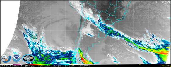
Let’s use a NetCDF with another domain. Please download this NetCDF sample from SMN Argentina. They receive it from PDA, and it is subsected on their region of interest.

Run the script with their file, changing the file name as appropriate. This should be the result:

The new remap file also works for mesoscales. For the plot below, we have used a sample downloaded from Amazon at this link. Try it out! Do not forget to adjust the colorbar and logo position.

GOES-16 data posted on this page are preliminary, non-operational and are undergoing testing